We consider the numerical solution of a parabolic partial differential equation in two spatial dimensions. Let $\Omega = [x_{\min}, x_{\max}] \times [y_{\min}, y_{\max}]$ and let $u : \Omega \times [0, T] \to \mathbb{R}$ satisfy
\[\frac{\partial u}{\partial t} = \sigma_{xx}(x,y,t)\frac{\partial^2 u}{\partial x^2} + 2\,\sigma_{xy}(x,y,t)\frac{\partial^2 u}{\partial x\,\partial y} + \sigma_{yy}(x,y,t)\frac{\partial^2 u}{\partial y^2} + F(x,y,t),\]subject to prescribed initial and boundary conditions, where we assume the diffusion matrix $\begin{pmatrix} \sigma_{xx} & \sigma_{xy} \ \sigma_{xy} & \sigma_{yy} \end{pmatrix}$ is symmetric positive definite everywhere so that the PDE is parabolic. The term $F(x,y,t)$ is an optional space- and time-dependent forcing; it is zero when omitted.
We discretize $\Omega$ with a uniform Cartesian grid of $N_x \times N_y$ interior points with mesh spacings $h_x$ and $h_y$, and collect the unknowns in lexicographic order to obtain the system of ODEs
\[\frac{d U(t)}{dt} = A(t)\,U(t) + F(t), \qquad U(0) = U_0,\]where $U(t) \in \mathbb{R}^{N_x N_y}$, $A(t) \in \mathbb{R}^{N_x N_y \times N_x N_y}$, and $F(t) \in \mathbb{R}^{N_x N_y}$ is the discretised forcing. Our goal is to explore efficient methods for solving this equation, called alternating direction implicit (ADI) methods.
The first step is to discretize the time derivative using the $\vartheta$-method. Introducing a uniform partition $t_0 = 0 < t_1 < \cdots < t_N = T$ with step $\Delta t$, the scheme reads
\[\frac{U^{(n+1)} - U^{(n)}}{\Delta t} = \vartheta \bigl[A^{(n+1)} U^{(n+1)} + F^{(n+1)}\bigr] + (1 - \vartheta)\,\bigl[A^{(n)} U^{(n)} + F^{(n)}\bigr],\]where $U^{(n)} := U(t_n)$, $A^{(n)} := A(t_n)$, and $F^{(n)} := F(t_n)$. With $\vartheta = 0$ the scheme is the explicit Euler method; with $\vartheta = 1$ it is the implicit Euler method; with $\vartheta = 1/2$ it is the Crank–Nicolson method.
Local truncation error. To assess accuracy, substitute the exact solution into the scheme. On the left-hand side, a Taylor expansion gives \(\frac{U(t_{n+1}) - U(t_n)}{\Delta t} = U'(t_n) + \frac{\Delta t}{2}\,U''(t_n) + \mathcal{O}(\Delta t^2).\) On the right-hand side, expanding $A(t_{n+1})U(t_{n+1}) + F(t_{n+1})$ around $t_n$: \(\vartheta \bigl[A^{(n+1)} U^{(n+1)} + F^{(n+1)}\bigr] + (1-\vartheta)\bigl[A^{(n)} U^{(n)} + F^{(n)}\bigr] = A^{(n)} U^{(n)} + F^{(n)} + \vartheta \Delta t \frac{d}{dt}\!\bigl[A(t)U(t)+F(t)\bigr]_{t_n} + \mathcal{O}(\Delta t^2).\) Since $U’(t_n) = A^{(n)} U^{(n)} + F^{(n)}$, the residual upon substitution is \(\left(\tfrac{1}{2} - \vartheta\right)\Delta t\, U''(t_n) + \mathcal{O}(\Delta t^2).\) The scheme is therefore first-order accurate ($\mathcal{O}(\Delta t)$ global error) for any $\vartheta \neq 1/2$, and second-order accurate for $\vartheta = 1/2$.
Rearranging to isolate $U^{(n+1)}$ gives
\[[I - \vartheta \Delta t A^{(n+1)}] U^{(n+1)} = [I + (1-\vartheta)\,\Delta t A^{(n)}] U^{(n)} + \Delta t\bigl[\vartheta F^{(n+1)} + (1-\vartheta) F^{(n)}\bigr] + \mathcal{O}(\Delta t^2).\tag{$*$}\]We now exploit the structure of the spatial discretization. After applying standard second-order finite differences, the scaled matrix $\Delta t A(t)$ decomposes as
\[\Delta t\,A^{(n)} = A_0^{(n)} + A_1^{(n)} + A_2^{(n)},\]where each $A_i^{(n)} = \mathcal{O}(\Delta t)$ as $\Delta t \to 0$, and:
- $A_1^{(n)}$ collects the $x$-derivative terms. Using the standard three-point stencil for $\partial^2/\partial x^2$, after lexicographic ordering this matrix has the Kronecker product structure $A_1^{(n)} = \Delta t\,B_x^{(n)} \otimes I_{N_y}$, where $B_x^{(n)} \in \mathbb{R}^{N_x \times N_x}$ is tridiagonal.
- $A_2^{(n)}$ collects the $y$-derivative terms and satisfies $A_2^{(n)} = \Delta t\,I_{N_x} \otimes B_y^{(n)}$, where $B_y^{(n)} \in \mathbb{R}^{N_y \times N_y}$ is tridiagonal.
- $A_0^{(n)}$ collects the mixed-derivative terms ($\partial^2/\partial x\,\partial y$). This matrix does not admit a Kronecker product structure.
The Kronecker structure of $A_1$ and $A_2$ is the key property for the ADI method: the linear system $(I - \vartheta A_1)v = r$ decouples into $N_y$ independent tridiagonal systems of size $N_x$, each solvable in $\mathcal{O}(N_x)$ operations by Thomas’s algorithm, for a total cost of $\mathcal{O}(N_x N_y)$. The same holds for $(I - \vartheta A_2)$. By contrast, solving $(I - \vartheta A_1 - \vartheta A_2)v = r$ directly would require $\mathcal{O}((N_x N_y)^3)$ operations.
Assumption. We require that $\sigma_{xx}, \sigma_{yy} > 0$ uniformly, so that $B_x$ and $B_y$ are non-singular M-matrices and $(I - \vartheta A_i)$ is invertible for all $\Delta t > 0$ and $\vartheta \in [0,1]$.
Explicit treatment of mixed derivatives. To preserve the efficient Kronecker structure, we treat $A_0$ explicitly: it is evaluated only at the known time level $t_n$ and placed on the right-hand side. This is an implicit–explicit (IMEX) splitting in which only $A_1$ and $A_2$ are handled implicitly.
The error introduced by this choice is bounded as follows. The full $\vartheta$-method would treat $A_0$ with coefficient $\vartheta$ implicitly and $(1-\vartheta)$ explicitly; the IMEX scheme treats it entirely explicitly. The difference, relative to a fully implicit treatment, is \(\vartheta\!\left[A_0^{(n+1)} U^{(n+1)} - A_0^{(n)} U^{(n)}\right].\) Writing $A_0^{(n+1)} U^{(n+1)} - A_0^{(n)} U^{(n)} = (A_0^{(n+1)} - A_0^{(n)}) U^{(n+1)} + A_0^{(n)}(U^{(n+1)} - U^{(n)})$, and using $A_0^{(n+1)} - A_0^{(n)} = \mathcal{O}(\Delta t^2)$ (since $A_0 = \mathcal{O}(\Delta t)$ changes smoothly in time) and $U^{(n+1)} - U^{(n)} = \mathcal{O}(\Delta t)$, this difference is $\mathcal{O}(\Delta t^2)$ — the same order as the local truncation error of the $\vartheta$-method. Hence the IMEX treatment of $A_0$ does not reduce the overall accuracy of the scheme.
Stability. The explicit treatment of $A_0$ imposes an additional stability constraint, analogous to a CFL condition on the mixed-derivative term. If $\sigma_{xy}$ is small relative to $\sigma_{xx}$ and $\sigma_{yy}$, this constraint is mild. In the important special case $\sigma_{xy} = 0$, we have $A_0 = 0$ and no stability restriction arises.
Substituting the decomposition $\Delta t\,A^{(n)} = A_0^{(n)} + A_1^{(n)} + A_2^{(n)}$ into the $\vartheta$-method and applying the IMEX splitting, the scheme becomes
\[[I - \vartheta A_1^{(n+1)} - \vartheta A_2^{(n+1)}] U^{(n+1)} = [I + A_0^{(n)} + (1-\vartheta) A_1^{(n)} + (1-\vartheta)\,A_2^{(n)}] U^{(n)} + \Delta t\,[\vartheta F^{(n+1)} + (1-\vartheta)\,F^{(n)}] + \mathcal{O}(\Delta t^3).\]Error accounting. Two sources contribute to the $\mathcal{O}(\Delta t^3)$ remainder in the scaled notation:
- The local truncation error of the $\vartheta$-method is $\mathcal{O}(\Delta t^2)$ in absolute terms; since each $A_i = \mathcal{O}(\Delta t)$, this is $\mathcal{O}(\Delta t^3)$ when measured in units of $A_i$.
- The IMEX approximation of $A_0$ contributes $\mathcal{O}(\Delta t^2)$ in absolute terms, which is likewise $\mathcal{O}(\Delta t^3)$ in the scaled notation.
The left-hand side contains the sum $I - \vartheta A_1 - \vartheta A_2$, which cannot be factored into independent tridiagonal operators. The next step addresses this by introducing an $\mathcal{O}(\Delta t^3)$ perturbation that enables a clean factorization.
We observe the algebraic identity
\[(I - \vartheta A_1)(I - \vartheta A_2) = I - \vartheta A_1 - \vartheta A_2 + \vartheta^2 A_1 A_2.\]Adding $\vartheta^2 A_1^{(n+1)} A_2^{(n+1)} U^{(n+1)}$ to both sides of the previous equation, the left-hand side becomes the product $(I - \vartheta A_1^{(n+1)})(I - \vartheta A_2^{(n+1)}) U^{(n+1)}$. The same term must be added to the right-hand side; we approximate it at time level $n$ and collect the difference as an additional error:
\[\begin{align*} & (I - \vartheta A_1^{(n+1)})(I - \vartheta A_2^{(n+1)}) U^{(n+1)} = \\ & \quad\quad [I + A_0^{(n)} + (1-\vartheta) A_1^{(n)} + (1-\vartheta) A_2^{(n)} + \vartheta^2 A_1^{(n)} A_2^{(n)}] U^{(n)} \\ & \quad\quad + \Delta t\,[\vartheta F^{(n+1)} + (1-\vartheta)\,F^{(n)}] \\ & \quad\quad + \vartheta^2 A_1^{(n+1)} A_2^{(n+1)} U^{(n+1)} - \vartheta^2 A_1^{(n)} A_2^{(n)} U^{(n)} + \mathcal{O}(\Delta t^3). \end{align*}\]Absorbing the cross-term residual. The difference $A_1^{(n+1)} A_2^{(n+1)} U^{(n+1)} - A_1^{(n)} A_2^{(n)} U^{(n)}$ is $\mathcal{O}(\Delta t^3)$ in the scaled notation. To see this, write
\[A_1^{(n+1)} A_2^{(n+1)} U^{(n+1)} - A_1^{(n)} A_2^{(n)} U^{(n)} = (A_1^{(n+1)} - A_1^{(n)}) A_2^{(n+1)} U^{(n+1)} + A_1^{(n)} (A_2^{(n+1)} - A_2^{(n)}) U^{(n+1)} + A_1^{(n)} A_2^{(n)} (U^{(n+1)} - U^{(n)}).\]Each $A_i^{(n)} = \mathcal{O}(\Delta t)$; each difference $A_i^{(n+1)} - A_i^{(n)} = \mathcal{O}(\Delta t^2)$ (since $A_i = \Delta t \hat{A}_i(t)$ with $\hat{A}_i$ smooth); and $U^{(n+1)} - U^{(n)} = \mathcal{O}(\Delta t)$. The three terms are therefore $\mathcal{O}(\Delta t^2)\cdot\mathcal{O}(\Delta t)$, $\mathcal{O}(\Delta t)\cdot\mathcal{O}(\Delta t^2)$, and $\mathcal{O}(\Delta t)\cdot\mathcal{O}(\Delta t)\cdot\mathcal{O}(\Delta t)$, all equal to $\mathcal{O}(\Delta t^3)$. Multiplying by $\vartheta^2$ leaves the order unchanged, so the residual is absorbed into the existing $\mathcal{O}(\Delta t^3)$ term, yielding the factored scheme:
\[(I - \vartheta A_1^{(n+1)})(I - \vartheta A_2^{(n+1)}) U^{(n+1)} = [I + A_0^{(n)} + (1-\vartheta) A_1^{(n)} + (1-\vartheta) A_2^{(n)} + \vartheta^2 A_1^{(n)} A_2^{(n)}] U^{(n)} + \Delta t\,[\vartheta F^{(n+1)} + (1-\vartheta)\,F^{(n)}] + \mathcal{O}(\Delta t^3).\]Two-step splitting. We now split the factored equation into two sequential solves. Define the intermediate variable
\[Y^\star := (I - \vartheta A_2^{(n+1)}) U^{(n+1)} + \vartheta A_2^{(n+1)} U^{(n)}.\]Applying $(I - \vartheta A_1^{(n+1)})$ to $Y^\star$ and expanding:
\[\begin{align*} (I - \vartheta A_1^{(n+1)}) Y^\star &= (I - \vartheta A_1^{(n+1)})(I - \vartheta A_2^{(n+1)}) U^{(n+1)} + (I - \vartheta A_1^{(n+1)}) \vartheta A_2^{(n+1)} U^{(n)}. \end{align*}\]Substituting the factored scheme into the first term, and expanding the second term as $\vartheta A_2^{(n+1)} U^{(n)} - \vartheta^2 A_1^{(n+1)} A_2^{(n+1)} U^{(n)}$, then using $A_2^{(n+1)} = A_2^{(n)} + \mathcal{O}(\Delta t^2)$ and $\vartheta^2 A_1^{(n)} A_2^{(n)} = \mathcal{O}(\Delta t^2)$:
\[\begin{align*} (I - \vartheta A_1^{(n+1)}) Y^\star &= [I + A_0^{(n)} + (1-\vartheta) A_1^{(n)} + (1-\vartheta) A_2^{(n)} + \vartheta^2 A_1^{(n)} A_2^{(n)}] U^{(n)} \\ &\quad + \Delta t\,[\vartheta F^{(n+1)} + (1-\vartheta)\,F^{(n)}] \\ &\quad + \vartheta A_2^{(n)} U^{(n)} - \vartheta^2 A_1^{(n)} A_2^{(n)} U^{(n)} + \mathcal{O}(\Delta t^3) \\ &= [I + A_0^{(n)} + (1-\vartheta) A_1^{(n)} + A_2^{(n)}] U^{(n)} + \Delta t\,[\vartheta F^{(n+1)} + (1-\vartheta)\,F^{(n)}] + \mathcal{O}(\Delta t^3), \end{align*}\]where in the last step we combined $(1-\vartheta) A_2^{(n)} + \vartheta A_2^{(n)} = A_2^{(n)}$ and $\vartheta^2 A_1^{(n)} A_2^{(n)} - \vartheta^2 A_1^{(n)} A_2^{(n)} = 0$. This gives the Douglas–Rachford ADI scheme:
\[\begin{align*} (I - \vartheta A_1^{(n+1)}) Y^\star &= \left[I + A_0^{(n)} + (1-\vartheta) A_1^{(n)} + A_2^{(n)}\right] U^{(n)} + \Delta t\,[\vartheta F^{(n+1)} + (1-\vartheta)\,F^{(n)}], \\ (I - \vartheta A_2^{(n+1)}) U^{(n+1)} &= Y^\star - \vartheta A_2^{(n+1)} U^{(n)}. \end{align*}\]The right-hand side of the first equation is fully known at time $t_n$. The first solve involves $(I - \vartheta A_1^{(n+1)})$, which decomposes into $N_y$ independent tridiagonal systems of size $N_x$. The second solve involves $(I - \vartheta A_2^{(n+1)})$, which decomposes into $N_x$ independent tridiagonal systems of size $N_y$. The total cost per time step is $\mathcal{O}(N_x N_y)$, compared to $\mathcal{O}((N_x N_y)^3)$ for a monolithic implicit solve.
Limitations of Douglas–Rachford and the need for extensions. DR treats the mixed-derivative term $A_0$ explicitly throughout: the only information about $A_0$ that enters is $A_0^{(n)} U^{(n)}$ on the right-hand side of step 1. This has two consequences. First, order: the one-sided explicit treatment makes DR only first-order accurate once $A_0 \neq 0$; it is second-order only in the mixed-derivative-free case $A_0 = 0$ (with $\vartheta = \tfrac12$). Second, stability: when $\sigma_{xy}$ is non-negligible the eigenvalues of $A_0$ can be large and of mixed sign, and the explicit treatment requires a step-size restriction of the form
\[\Delta t \leq \frac{C}{\|\sigma_{xy}\|^2 / (\sigma_{xx}\,\sigma_{yy})},\]analogous to a CFL condition on the mixed part. This is harmless when $\sigma_{xy} \approx 0$ but becomes binding in applications — such as multi-asset option pricing — where correlations close to $\pm 1$ make $\sigma_{xy}$ comparable to $\sigma_{xx}$ and $\sigma_{yy}$.
The three extensions below each restore second-order accuracy for $A_0 \neq 0$ and enlarge the stability region. All three share the DR predictor and add a second ADI pass (a corrector) — so they cost twice the tridiagonal solves of DR — differing only in how the corrector’s right-hand side is assembled:
- Craig–Sneyd (CS): the corrector replaces the mixed term by its trapezoidal average.
- Modified Craig–Sneyd (MCS): as CS, plus a $(\tfrac12-\vartheta)$ increment of the full operator; identical to CS at $\vartheta = \tfrac12$, more robust for $\vartheta \neq \tfrac12$.
- Hundsdorfer–Verwer (HV): the corrector uses the trapezoidal average of the entire right-hand side, giving unconditional stability for all $\sigma_{xy}$.
Craig–Sneyd scheme (CS). In the full $\vartheta$-method the mixed term contributes the balanced average $\vartheta A_0^{(n+1)} U^{(n+1)} + (1-\vartheta) A_0^{(n)} U^{(n)}$, whereas the DR predictor carries only $A_0^{(n)} U^{(n)}$. CS restores the balance by recomputing $U^{(n+1)}$ from a second ADI pass whose right-hand side has the mixed term replaced by its trapezoidal average.
Write the explicit step-1 right-hand side of the predictor as \(R := \bigl[I + A_0^{(n)} + (1-\vartheta) A_1^{(n)} + A_2^{(n)}\bigr]\,U^{(n)} + \Delta t\,[\vartheta F^{(n+1)} + (1-\vartheta)\,F^{(n)}].\) Then DR is the predictor (steps 1–2) and CS appends the corrector (steps 3–4): \(\begin{align*} (I - \vartheta A_1^{(n+1)})\,Y^\star &= R, & (I - \vartheta A_2^{(n+1)})\,\tilde{U}^{(n+1)} &= Y^\star - \vartheta A_2^{(n+1)}\,U^{(n)}, \\[4pt] (I - \vartheta A_1^{(n+1)})\,\tilde{Y}^\star &= R + \tfrac{1}{2}\bigl[A_0^{(n+1)}\tilde{U}^{(n+1)} - A_0^{(n)} U^{(n)}\bigr], & (I - \vartheta A_2^{(n+1)})\,U^{(n+1)} &= \tilde{Y}^\star - \vartheta A_2^{(n+1)}\,U^{(n)}. \end{align*}\)
The corrector reuses $R$ (which already contains $A_0^{(n)} U^{(n)}$) and adds $\tfrac{1}{2}\bigl[A_0^{(n+1)}\tilde{U}^{(n+1)} - A_0^{(n)} U^{(n)}\bigr]$, so the net mixed-term contribution becomes the trapezoidal average $\tfrac{1}{2}\bigl[A_0^{(n)} U^{(n)} + A_0^{(n+1)}\tilde{U}^{(n+1)}\bigr]$. Crucially, this correction passes through the implicit sweeps rather than being added explicitly to $\tilde{U}^{(n+1)}$ — that is what keeps CS stable for $\sigma_{xy} \neq 0$. (A bare explicit $A_0$-correction, with no second solve, is unstable as soon as $A_0$ is non-trivial.)
| What we gain. CS extends the unconditional-stability region relative to DR, tolerating larger $ | \sigma_{xy} | /\sqrt{\sigma_{xx}\,\sigma_{yy}}$. |
What we lose. A second ADI pass: two extra tridiagonal solves per step, roughly doubling the DR cost. For $A_0 = 0$ the correction vanishes and CS reduces exactly to DR.
Modified Craig–Sneyd scheme (MCS). CS only balances the mixed term in the corrector. MCS additionally blends in a $(\tfrac{1}{2}-\vartheta)$ increment of the full operator, which improves the stability balance when $\vartheta \neq \tfrac{1}{2}$. The predictor is unchanged (same $R$ and $\tilde{U}^{(n+1)}$ as DR/CS); only the corrector’s right-hand side changes. Writing the one-step change of the complete right-hand side $\Phi(t,v) = (A_0+A_1+A_2)v + \Delta t\,F$ as \(\Delta\Phi := \Phi\bigl(t_{n+1}, \tilde{U}^{(n+1)}\bigr) - \Phi\bigl(t_n, U^{(n)}\bigr), \qquad \Delta A_0 := A_0^{(n+1)}\tilde{U}^{(n+1)} - A_0^{(n)} U^{(n)},\) the corrector reads \(\begin{align*} (I - \vartheta A_1^{(n+1)})\,\tilde{Y}^\star &= R + \vartheta\,\Delta A_0 + \bigl(\tfrac{1}{2}-\vartheta\bigr)\,\Delta\Phi, \\ (I - \vartheta A_2^{(n+1)})\,U^{(n+1)} &= \tilde{Y}^\star - \vartheta A_2^{(n+1)}\,U^{(n)}. \end{align*}\)
Relation to CS. At $\vartheta = \tfrac{1}{2}$ the term $(\tfrac{1}{2}-\vartheta)\,\Delta\Phi$ vanishes and the mixed-term coefficient $\vartheta = \tfrac12$ matches CS exactly, so MCS and CS coincide. They differ only for $\vartheta \neq \tfrac{1}{2}$. Since every example here uses $\vartheta = \tfrac{1}{2}$, MCS and CS will produce identical numbers below.
| What we gain. For the relevant $\vartheta \neq \tfrac12$ regimes, MCS achieves unconditional stability over a substantially wider range of $ | \sigma_{xy} | /\sqrt{\sigma_{xx}\,\sigma_{yy}}$ than CS. |
What we lose. Nothing relative to CS: the cost is identical (a second ADI pass). The corrector right-hand side carries two extra matrix–vector products (for $\Delta\Phi$).
| Hundsdorfer–Verwer scheme (HV). When $ | \sigma_{xy} | $ is large (high correlations), MCS can still exhibit conditional stability. The HV scheme (Hundsdorfer & Verwer, 1995; In ‘t Hout & Welfert, 2007) achieves provable unconditional stability for all parameter values. Like CS and MCS it adds a second ADI pass to the DR predictor, but the corrector’s right-hand side is the trapezoidal average of the entire operator, and the corrector sweeps subtract the explicit terms at the predictor (new time level). |
Predictor (identical to DR), with explicit step-1 right-hand side $R$ as above: \((I - \vartheta A_1^{(n+1)})\,Y^\star = R, \qquad (I - \vartheta A_2^{(n+1)})\,\tilde{U}^{(n+1)} = Y^\star - \vartheta A_2^{(n+1)}\,U^{(n)}.\)
Corrected right-hand side. Let $\Phi(t,v)$ denote the complete discretised right-hand side of the ODE, \(\Phi(t,v) := \bigl(A_0(t) + A_1(t) + A_2(t)\bigr)\,v + \Delta t\,F(t),\) i.e. the full spatial operator (mixed plus both unidirectional parts) acting on $v$, plus the source. The HV corrector starts from the trapezoidal average of $\Phi$ at the old state and the predictor: \(\tilde{R} = U^{(n)} + \tfrac{1}{2}\Bigl[\Phi\bigl(t_n, U^{(n)}\bigr) + \Phi\bigl(t_{n+1}, \tilde{U}^{(n+1)}\bigr)\Bigr].\)
It is essential that $\tilde{R}$ uses the full operator $A_0 + A_1 + A_2$, not the mixed term $A_0$ alone. The trapezoidal average of the entire right-hand side is what lifts the corrector to second order; dropping $A_1 + A_2$ leaves it inconsistent, and the iteration then converges to the wrong solution (a flat, non-decreasing error under refinement).
Corrector (second pair of tridiagonal sweeps): \(\begin{align*} (I - \vartheta A_1^{(n+1)})\,\tilde{Y}^\star &= \tilde{R} - \vartheta A_1^{(n+1)}\,\tilde{U}^{(n+1)}, \\ (I - \vartheta A_2^{(n+1)})\,U^{(n+1)} &= \tilde{Y}^\star - \vartheta A_2^{(n+1)}\,\tilde{U}^{(n+1)}. \end{align*}\) Each implicit sweep removes the explicit $A_j^{(n+1)}$ contribution already contained in $\tilde{R}$, evaluated at the predictor $\tilde{U}^{(n+1)}$ (the new time level), not at $U^{(n)}$. With $\sigma_{xy} = 0$ and no forcing, $\tilde{R}$ reduces to a midpoint $\tfrac{1}{2}(U^{(n)} + \tilde{U}^{(n+1)})$ plus the diffusion increment, and the corrector becomes a second consistent ADI pass.
| What we gain. Unconditional stability for all values of $\sigma_{xy}$, regardless of the ratio $ | \sigma_{xy} | /\sqrt{\sigma_{xx}\,\sigma_{yy}}$. |
What we lose. Nothing in cost relative to CS/MCS — the same second ADI pass (twice the DR solves). The only difference is that HV subtracts the explicit terms at $\tilde U^{(n+1)}$ rather than at $U^{(n)}$, and assembles $\tilde R$ from the full operator.
Summary. The four schemes form a natural hierarchy. The three correctors all cost a second ADI pass (twice the DR solves); what that buys is higher order for $A_0 \neq 0$ and a progressively wider unconditional-stability region.
| Scheme | Tridiag. solves | Corrector RHS | Unconditionally stable | Order ($\vartheta = \tfrac{1}{2}$) |
|---|---|---|---|---|
| Douglas–Rachford | 2 | — | Only if $A_0 = 0$ | 2nd if $A_0=0$, else 1st |
| Craig–Sneyd | 4 | trapezoidal $A_0$ | Partial | 2nd |
| Modified Craig–Sneyd | 4 | trapezoidal $A_0$ + $(\tfrac12-\vartheta)$ full | Wider range | 2nd |
| Hundsdorfer–Verwer | 4 | trapezoidal full operator | Yes | 2nd |
| When $\sigma_{xy} = 0$ all four coincide (every corrector reduces to a second consistent ADI pass and DR is already second-order). At $\vartheta = \tfrac{1}{2}$, CS and MCS are identical. The practical choice depends on $ | \sigma_{xy} | /\sqrt{\sigma_{xx}\,\sigma_{yy}}$: CS/MCS suffice for moderate correlations, while HV is the safe default for strongly correlated problems. |
import numpy as np


class Grid2D:
    """
    Rectangular 2D grid, uniform or non-uniform.

    All grid points (including boundaries) are stored.  Interior points
    are indices 1 .. nx-2 in x and 1 .. ny-2 in y.

    Parameters
    ----------
    x, y : array-like
        Strictly increasing 1-D arrays of grid coordinates.
    """

    def __init__(self, x, y):
        self.x  = np.asarray(x, dtype=float)
        self.y  = np.asarray(y, dtype=float)
        self.nx = len(self.x)
        self.ny = len(self.y)
        self.hx = np.diff(self.x)          # (nx-1,)  spacings in x
        self.hy = np.diff(self.y)          # (ny-1,)  spacings in y
        # 2-D meshgrid evaluated with 'ij' ordering so shape is (nx, ny)
        self.X, self.Y = np.meshgrid(self.x, self.y, indexing='ij')

    @classmethod
    def uniform(cls, x0, x1, nx, y0, y1, ny):
        return cls(np.linspace(x0, x1, nx), np.linspace(y0, y1, ny))

    @classmethod
    def nonuniform(cls, x, y):
        return cls(x, y)


class Problem2D:
    """
    Coefficients and optional forcing for the PDE

        du/dt = sigma_xx * d²u/dx²  +  2 sigma_xy * d²u/dxdy  +  sigma_yy * d²u/dy²  +  f(x, y, t)

    Each coefficient and the forcing are callables  g(x, y, t) -> scalar or broadcastable array.
    The forcing f is optional; if omitted the source term is identically zero.
    """

    def __init__(self, sigma_xx, sigma_xy, sigma_yy, f=None):
        self._sxx = sigma_xx
        self._sxy = sigma_xy
        self._syy = sigma_yy
        self._f   = f

    def coeffs(self, grid, t):
        """Return (sxx, sxy, syy) as (nx, ny) arrays at time t."""
        def _eval(fn):
            v = np.asarray(fn(grid.X, grid.Y, t), dtype=float)
            return np.broadcast_to(v, grid.X.shape).copy()
        return _eval(self._sxx), _eval(self._sxy), _eval(self._syy)

    def source(self, grid, t):
        """Return f(x, y, t) as an (nx, ny) array at time t, or zeros if no forcing."""
        if self._f is None:
            return np.zeros(grid.X.shape)
        v = np.asarray(self._f(grid.X, grid.Y, t), dtype=float)
        return np.broadcast_to(v, grid.X.shape).copy()
class ADISolver2D:
    """
    ADI solver for the 2D parabolic PDE defined by a Problem2D on a Grid2D,
    with homogeneous Dirichlet boundary conditions.

    The source term F(x,y,t) in Problem2D is treated with the theta-method:
    the step-1 RHS receives  dt * ((1-theta)*F^n + theta*F^{n+1}).  It is masked
    to the interior (see _source) so the homogeneous Dirichlet data survives the
    directional solves even when F does not vanish on the boundary.

    DR is the bare Douglas predictor; CS, MCS and HV each add a second ADI pass
    (a corrector), so they cost twice the tridiagonal solves of DR.  For
    theta = 1/2, CS and MCS coincide.

    All four schemes are composed from the same five building blocks:

        Matrix-vector products (cheap, fully vectorised)
        ------------------------------------------------
        _apply_A1  :  sigma_xx * d²/dx²     applied to U
        _apply_A2  :  sigma_yy * d²/dy²     applied to U
        _apply_A0  :  2*sigma_xy * d²/dxdy  applied to U

        Tridiagonal solves  (vectorised Thomas algorithm)
        -------------------------------------------------
        _solve_A1  :  solve  (I - theta*dt*A1) X = rhs,  ny systems in x
        _solve_A2  :  solve  (I - theta*dt*A2) X = rhs,  nx systems in y

    Schemes
    -------
    step_DR   Douglas-Rachford
    step_CS   Craig-Sneyd
    step_MCS  Modified Craig-Sneyd
    step_HV   Hundsdorfer-Verwer
    """

    def __init__(self, grid: Grid2D, problem: Problem2D, theta: float = 0.5):
        self.grid    = grid
        self.problem = problem
        self.theta   = theta

    # ------------------------------------------------------------------ #
    #  Building blocks 1-3:  matrix-vector products                       #
    # ------------------------------------------------------------------ #

    def _apply_A1(self, U, sxx):
        """sigma_xx * d²u/dx²  via second-order non-uniform FD (x-direction)."""
        hx     = self.grid.hx
        hm     = hx[:-1, np.newaxis]   # h_{i-1,i}, shape (nx-2, 1)
        hp     = hx[1:,  np.newaxis]   # h_{i,i+1}, shape (nx-2, 1)
        c      = 2.0 / (hm + hp)
        result = np.zeros_like(U)
        result[1:-1] = sxx[1:-1] * c * (
            U[2:]   / hp
          - U[1:-1] * (1/hp + 1/hm)
          + U[:-2]  / hm
        )
        return result

    def _apply_A2(self, U, syy):
        """sigma_yy * d²u/dy²  via second-order non-uniform FD (y-direction)."""
        hy     = self.grid.hy
        hm     = hy[:-1][np.newaxis, :]  # (1, ny-2)
        hp     = hy[1:] [np.newaxis, :]  # (1, ny-2)
        c      = 2.0 / (hm + hp)
        result = np.zeros_like(U)
        result[:, 1:-1] = syy[:, 1:-1] * c * (
            U[:, 2:]   / hp
          - U[:, 1:-1] * (1/hp + 1/hm)
          + U[:, :-2]  / hm
        )
        return result

    def _apply_A0(self, U, sxy):
        """2*sigma_xy * d²u/dxdy  via second-order central FD."""
        hx, hy = self.grid.hx, self.grid.hy
        dx     = (hx[:-1] + hx[1:])[:, np.newaxis]  # (nx-2, 1)
        dy     = (hy[:-1] + hy[1:])[np.newaxis, :]  # (1,  ny-2)
        d2u    = (  U[2:,  2:] - U[:-2, 2:]
                  - U[2:, :-2] + U[:-2, :-2] ) / (dx * dy)
        result = np.zeros_like(U)
        result[1:-1, 1:-1] = 2.0 * sxy[1:-1, 1:-1] * d2u
        return result

    # ------------------------------------------------------------------ #
    #  Building blocks 4-5:  tridiagonal solves via vectorised Thomas     #
    # ------------------------------------------------------------------ #

    @staticmethod
    def _thomas(lower, diag, upper, rhs):
        """
        Solve m tridiagonal systems of size n simultaneously.

        Parameters: lower, diag, upper, rhs all have shape (n, m).
        lower[0] and upper[-1] are not referenced.
        Returns x of shape (n, m).
        """
        n = diag.shape[0]
        u = upper.copy()
        d = rhs.copy()
        b = diag.copy()
        for i in range(1, n):
            w     = lower[i] / b[i - 1]
            b[i] -= w * u[i - 1]
            d[i] -= w * d[i - 1]
        x     = np.empty_like(d)
        x[-1] = d[-1] / b[-1]
        for i in range(n - 2, -1, -1):
            x[i] = (d[i] - u[i] * x[i + 1]) / b[i]
        return x

    def _solve_A1(self, rhs, sxx, dt):
        """
        Solve  (I - theta*dt*sigma_xx*d²/dx²) X = rhs.

        Tridiagonal in x; ny systems solved simultaneously via Thomas.
        """
        th, hx = self.theta, self.grid.hx
        nx, ny = self.grid.nx, self.grid.ny
        hm = hx[:-1, np.newaxis]                       # (nx-2, 1)
        hp = hx[1:,  np.newaxis]                       # (nx-2, 1)
        c  = th * dt * sxx[1:-1] * 2.0 / (hm + hp)   # (nx-2, ny)

        lower = np.zeros((nx, ny));  lower[1:-1] = -c / hm
        diag  = np.ones ((nx, ny));  diag [1:-1] =  1.0 + c * (1/hm + 1/hp)
        upper = np.zeros((nx, ny));  upper[1:-1] = -c / hp
        return self._thomas(lower, diag, upper, rhs)

    def _solve_A2(self, rhs, syy, dt):
        """
        Solve  (I - theta*dt*sigma_yy*d²/dy²) X = rhs.

        Tridiagonal in y; nx systems solved simultaneously via Thomas.
        Arrays are transposed so the Thomas loop iterates over y.
        """
        th, hy = self.theta, self.grid.hy
        nx, ny = self.grid.nx, self.grid.ny
        hm = hy[:-1][np.newaxis, :]                    # (1, ny-2)
        hp = hy[1:] [np.newaxis, :]                    # (1, ny-2)
        c  = th * dt * syy[:, 1:-1] * 2.0 / (hm + hp) # (nx, ny-2)

        lower = np.zeros((ny, nx));  lower[1:-1] = (-c / hm).T
        diag  = np.ones ((ny, nx));  diag [1:-1] = (1.0 + c * (1/hm + 1/hp)).T
        upper = np.zeros((ny, nx));  upper[1:-1] = (-c / hp).T
        return self._thomas(lower, diag, upper, rhs.T).T

    # ------------------------------------------------------------------ #
    #  Schemes  (thin compositions of the five building blocks above)     #
    # ------------------------------------------------------------------ #

    def _source(self, t):
        """Forcing f(.,t) as an (nx,ny) array with its boundary values zeroed.

        The operator blocks _apply_A0/A1/A2 already vanish on the boundary, so
        masking the source here is what preserves the homogeneous Dirichlet data
        through the directional solves.  A forcing that does not itself vanish on
        the boundary (e.g. the one for a mixed-derivative manufactured solution)
        would otherwise leak dt*f into the boundary nodes and, through the
        tridiagonal solves, into the interior -- destroying consistency.
        """
        f = self.problem.source(self.grid, t)
        f[0, :] = f[-1, :] = f[:, 0] = f[:, -1] = 0.0
        return f

    def _predict(self, U, t, dt):
        """Douglas predictor, shared by all four schemes.

        Returns (rhs0, U_pred): rhs0 is the explicit step-1 right-hand side and
        U_pred is the Douglas-Rachford estimate of U^{n+1}.
        """
        th = self.theta
        sxx0, sxy0, syy0 = self.problem.coeffs(self.grid, t)
        sxx1, sxy1, syy1 = self.problem.coeffs(self.grid, t + dt)
        f0, f1 = self._source(t), self._source(t + dt)

        rhs0   = U + dt * (  self._apply_A0(U, sxy0)
                            + (1 - th) * self._apply_A1(U, sxx0)
                            +            self._apply_A2(U, syy0)
                            + (1 - th) * f0 + th * f1)
        Ystar  = self._solve_A1(rhs0, sxx1, dt)
        U_pred = self._solve_A2(Ystar - th * dt * self._apply_A2(U, syy1), syy1, dt)
        return rhs0, U_pred

    def step_DR(self, U, t, dt):
        """Douglas-Rachford: the bare predictor."""
        return self._predict(U, t, dt)[1]

    def step_CS(self, U, t, dt):
        """Craig-Sneyd: predictor + a second ADI pass that adds the half-weighted
        mixed-derivative increment at the new time level.  The net treatment of
        A0 becomes the trapezoidal average 1/2 (A0^n U^n + A0^{n+1} U_pred)."""
        th = self.theta
        sxx0, sxy0, syy0 = self.problem.coeffs(self.grid, t)
        sxx1, sxy1, syy1 = self.problem.coeffs(self.grid, t + dt)
        rhs0, U_pred = self._predict(U, t, dt)

        rhs1  = rhs0 + 0.5 * dt * (  self._apply_A0(U_pred, sxy1)
                                   - self._apply_A0(U,      sxy0))
        Ystar = self._solve_A1(rhs1, sxx1, dt)
        return  self._solve_A2(Ystar - th * dt * self._apply_A2(U, syy1), syy1, dt)

    def step_MCS(self, U, t, dt):
        """Modified Craig-Sneyd: like CS, but the corrector also carries a
        (1/2 - theta) increment of the *full* operator.  For theta = 1/2 this
        term vanishes and MCS coincides exactly with CS; the two differ only for
        theta != 1/2, where MCS has the larger unconditional-stability region."""
        th = self.theta
        sxx0, sxy0, syy0 = self.problem.coeffs(self.grid, t)
        sxx1, sxy1, syy1 = self.problem.coeffs(self.grid, t + dt)
        f0, f1 = self._source(t), self._source(t + dt)
        rhs0, U_pred = self._predict(U, t, dt)

        A0_diff  = self._apply_A0(U_pred, sxy1) - self._apply_A0(U, sxy0)
        phi_diff = (  A0_diff
                    + self._apply_A1(U_pred, sxx1) - self._apply_A1(U, sxx0)
                    + self._apply_A2(U_pred, syy1) - self._apply_A2(U, syy0)
                    + f1 - f0)
        rhs1  = rhs0 + th * dt * A0_diff + (0.5 - th) * dt * phi_diff
        Ystar = self._solve_A1(rhs1, sxx1, dt)
        return  self._solve_A2(Ystar - th * dt * self._apply_A2(U, syy1), syy1, dt)

    def step_HV(self, U, t, dt):
        """Hundsdorfer-Verwer: predictor + a second ADI pass whose right-hand
        side is the trapezoidal average of the *full* operator (mixed +
        unidirectional + source).  Each implicit sweep removes the explicit
        A_j contribution evaluated at the predictor (the new time level)."""
        th = self.theta
        sxx0, sxy0, syy0 = self.problem.coeffs(self.grid, t)
        sxx1, sxy1, syy1 = self.problem.coeffs(self.grid, t + dt)
        f0, f1 = self._source(t), self._source(t + dt)
        _, U_pred = self._predict(U, t, dt)

        Phi_old = (  self._apply_A0(U, sxy0)
                   + self._apply_A1(U, sxx0)
                   + self._apply_A2(U, syy0) + f0)
        Phi_new = (  self._apply_A0(U_pred, sxy1)
                   + self._apply_A1(U_pred, sxx1)
                   + self._apply_A2(U_pred, syy1) + f1)
        R_tilde = U + 0.5 * dt * (Phi_old + Phi_new)

        Ystar = self._solve_A1(R_tilde - th * dt * self._apply_A1(U_pred, sxx1), sxx1, dt)
        return  self._solve_A2(Ystar  - th * dt * self._apply_A2(U_pred, syy1), syy1, dt)

    # ------------------------------------------------------------------ #
    #  Time-marching loop                                                  #
    # ------------------------------------------------------------------ #

    def solve(self, U0, t_span, dt, scheme='MCS'):
        """
        March from t_span[0] to t_span[1] with step dt.

        Parameters
        ----------
        U0     : (nx, ny) ndarray  — initial condition (boundary values must be 0)
        t_span : (t0, t_end)
        dt     : float
        scheme : 'DR' | 'CS' | 'MCS' | 'HV'
        """
        step_fn = {'DR':  self.step_DR,  'CS':  self.step_CS,
                   'MCS': self.step_MCS, 'HV':  self.step_HV}[scheme]
        t, t_end = float(t_span[0]), float(t_span[1])
        U = U0.copy()
        while t < t_end - 1e-14 * abs(dt):
            dt_eff = min(dt, t_end - t)
            U = step_fn(U, t, dt_eff)
            t += dt_eff
        return U
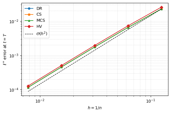
Example: isotropic heat equation with source term. We verify the implementation using the method of manufactured solutions. We solve
\[\frac{\partial u}{\partial t} = \frac{\partial^2 u}{\partial x^2} + \frac{\partial^2 u}{\partial y^2} + F(x,y,t), \qquad (x,y) \in [0,1]^2, \quad t \in [0, 1],\]with homogeneous Dirichlet boundary conditions. Choosing the exact solution
\[u(x,y,t) = \sin(\pi x)\sin(\pi y)\,e^{t},\]which satisfies zero Dirichlet conditions for all $t$, the required forcing is
\[F(x,y,t) = \frac{\partial u}{\partial t} - \frac{\partial^2 u}{\partial x^2} - \frac{\partial^2 u}{\partial y^2} = (1 + 2\pi^2)\,\sin(\pi x)\sin(\pi y)\,e^{t}.\]The solution grows exponentially in time rather than decaying, making it a more demanding test of the source term treatment. Here $\sigma_{xx} = \sigma_{yy} = 1$ and $\sigma_{xy} = 0$, so all four schemes should agree. We run a convergence study, halving $\Delta t$ and $h$ simultaneously, and verify second-order accuracy ($\vartheta = 1/2$).
import numpy as np
import matplotlib.pyplot as plt

# ---- Problem definition ------------------------------------------------
problem_iso = Problem2D(
    sigma_xx = lambda x, y, t: np.ones_like(x),
    sigma_xy = lambda x, y, t: np.zeros_like(x),
    sigma_yy = lambda x, y, t: np.ones_like(x),
    f        = lambda x, y, t: (1 + 2 * np.pi**2) * np.sin(np.pi * x) * np.sin(np.pi * y) * np.exp(t),
)

T      = 1.0
t_span = (0.0, T)

def exact_iso(grid, t):
    return np.sin(np.pi * grid.X) * np.sin(np.pi * grid.Y) * np.exp(t)

# ---- Convergence study -------------------------------------------------
schemes  = ['DR', 'CS', 'MCS', 'HV']
n_points = [8, 16, 32, 64, 128]

hs     = []
errors = {s: [] for s in schemes}

for n in n_points:
    grid   = Grid2D.uniform(0, 1, n + 2, 0, 1, n + 2)
    solver = ADISolver2D(grid, problem_iso, theta=0.5)
    U0     = exact_iso(grid, 0.0)
    U0[0, :] = U0[-1, :] = U0[:, 0] = U0[:, -1] = 0.0
    dt     = T / (4 * n)
    U_ex   = exact_iso(grid, T)
    hs.append(1.0 / n)
    for s in schemes:
        U_num = solver.solve(U0, t_span, dt, scheme=s)
        errors[s].append(np.max(np.abs(U_num - U_ex)))

hs = np.array(hs)

# ---- Plot --------------------------------------------------------------
fig, ax = plt.subplots(figsize=(6, 4))

colors  = ['C0', 'C1', 'C2', 'C3']
markers = ['o', 's', '^', 'D']

for s, c, m in zip(schemes, colors, markers):
    ax.loglog(hs, errors[s], marker=m, color=c, label=s, linewidth=1.5, markersize=5)

ref = errors['DR'][0] * (hs / hs[0])**2
ax.loglog(hs, ref, 'k--', linewidth=1, label=r'$\mathcal{O}(h^2)$')

ax.set_xlabel(r'$h = 1/n$')
ax.set_ylabel(r'$\ell^\infty$ error at $t = T$')
ax.legend(loc='upper left')
ax.grid(True, which='both', linestyle=':', linewidth=0.5)
plt.tight_layout()
plt.show()

# ---- Print table -------------------------------------------------------
print(f"\n{'n':>5}  {'h':>8}", end="")
for s in schemes:
    print(f"  {s+' err':>10}", end="")
print()
for k, n in enumerate(n_points):
    row = f"{n:>5}  {hs[k]:>8.4f}"
    for s in schemes:
        row += f"  {errors[s][k]:>10.2e}"
    print(row)

print(f"\n{'n':>5}  {'h':>8}", end="")
for s in schemes:
    print(f"  {s+' rate':>10}", end="")
print()
for k in range(1, len(n_points)):
    row = f"{n_points[k]:>5}  {hs[k]:>8.4f}"
    for s in schemes:
        rate = np.log2(errors[s][k - 1] / errors[s][k])
        row += f"  {rate:>10.2f}"
    print(row)
    n         h      DR err      CS err     MCS err      HV err
    8    0.1250    2.26e-02    2.26e-02    2.26e-02    2.56e-02
   16    0.0625    6.54e-03    6.54e-03    6.54e-03    7.31e-03
   32    0.0312    1.76e-03    1.76e-03    1.76e-03    1.95e-03
   64    0.0156    4.55e-04    4.55e-04    4.55e-04    5.04e-04
  128    0.0078    1.16e-04    1.16e-04    1.16e-04    1.28e-04

    n         h     DR rate     CS rate    MCS rate     HV rate
   16    0.0625        1.79        1.79        1.79        1.81
   32    0.0312        1.90        1.90        1.90        1.91
   64    0.0156        1.95        1.95        1.95        1.95
  128    0.0078        1.97        1.97        1.97        1.98
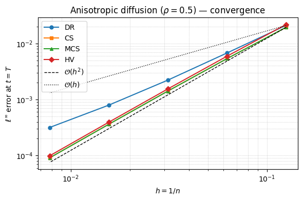
Example: anisotropic diffusion with mixed derivative. We now switch on $\sigma_{xy} \neq 0$, taking constant coefficients $\sigma_{xx} = \sigma_{yy} = 1$ and $\sigma_{xy} = \rho = 0.5$, and again verify with a manufactured solution. Keeping the same exact solution
\[u(x,y,t) = \sin(\pi x)\sin(\pi y)\,e^{t}, \qquad (x,y)\in[0,1]^2,\ t\in[0,1],\]the mixed derivative now contributes $u_{xy} = \pi^2\cos(\pi x)\cos(\pi y)\,e^{t}$, so the required forcing picks up a cosine term:
\[F(x,y,t) = u_t - u_{xx} - 2\rho\,u_{xy} - u_{yy} = (1 + 2\pi^2)\,\sin(\pi x)\sin(\pi y)\,e^{t} \;-\; 2\rho\,\pi^2\cos(\pi x)\cos(\pi y)\,e^{t}.\]Note that this $F$ does not vanish on the boundary (the cosine term is non-zero there), unlike the $\sigma_{xy}=0$ case. The solver applies the forcing on the interior only (ADISolver2D._source masks the boundary), which is what keeps the homogeneous Dirichlet data exact; without that masking the boundary nodes would absorb $\Delta t\,F$ and the global error would stop converging.
The convergence study below shows the expected hierarchy: DR drops to first order once the mixed term is present (its explicit one-sided treatment of $A_0$), while CS, MCS and HV remain second order. Because $\vartheta = \tfrac12$, CS and MCS coincide exactly.
rho = 0.5

# Manufactured solution u = sin(pi x) sin(pi y) e^t with the mixed term active.
# Forcing: F = u_t - u_xx - 2 rho u_xy - u_yy
#            = (1 + 2 pi^2) sin(pi x) sin(pi y) e^t  -  2 rho pi^2 cos(pi x) cos(pi y) e^t
problem_mixed = Problem2D(
    sigma_xx = lambda x, y, t: np.ones_like(x),
    sigma_xy = lambda x, y, t: rho * np.ones_like(x),
    sigma_yy = lambda x, y, t: np.ones_like(x),
    f        = lambda x, y, t: ((1 + 2 * np.pi**2) * np.sin(np.pi * x) * np.sin(np.pi * y)
                                - 2 * rho * np.pi**2 * np.cos(np.pi * x) * np.cos(np.pi * y)) * np.exp(t),
)

T      = 1.0
t_span = (0.0, T)

def exact_mixed(grid, t):
    return np.sin(np.pi * grid.X) * np.sin(np.pi * grid.Y) * np.exp(t)

# ---- Convergence study -------------------------------------------------
n_points = [8, 16, 32, 64, 128]
hs       = np.array([1.0 / n for n in n_points])
errors   = {s: [] for s in schemes}

for n in n_points:
    grid   = Grid2D.uniform(0, 1, n + 2, 0, 1, n + 2)
    solver = ADISolver2D(grid, problem_mixed, theta=0.5)
    U0     = exact_mixed(grid, 0.0)
    U0[0, :] = U0[-1, :] = U0[:, 0] = U0[:, -1] = 0.0
    dt     = T / (4 * n)
    U_ex   = exact_mixed(grid, T)
    for s in schemes:
        U_num = solver.solve(U0, t_span, dt, scheme=s)
        errors[s].append(np.max(np.abs(U_num - U_ex)))

# ---- Plot --------------------------------------------------------------
fig, ax = plt.subplots(figsize=(6, 4))

for s, c, m in zip(schemes, colors, markers):
    ax.loglog(hs, errors[s], marker=m, color=c, label=s, linewidth=1.5, markersize=5)

# Reference slopes anchored at the coarsest CS point
ref2 = errors['CS'][0] * (hs / hs[0])**2
ref1 = errors['DR'][0] * (hs / hs[0])
ax.loglog(hs, ref2, 'k--', linewidth=1, label=r'$\mathcal{O}(h^2)$')
ax.loglog(hs, ref1, 'k:',  linewidth=1, label=r'$\mathcal{O}(h)$')

ax.set_xlabel(r'$h = 1/n$')
ax.set_ylabel(r'$\ell^\infty$ error at $t = T$')
ax.set_title(rf'Anisotropic diffusion ($\rho={rho}$) — convergence')
ax.legend(loc='upper left')
ax.grid(True, which='both', linestyle=':', linewidth=0.5)
plt.tight_layout()
plt.show()

# ---- Print table -------------------------------------------------------
print(f"\n{'n':>5}  {'h':>8}", end="")
for s in schemes:
    print(f"  {s+' err':>10}", end="")
print()
for k, n in enumerate(n_points):
    row = f"{n:>5}  {hs[k]:>8.4f}"
    for s in schemes:
        row += f"  {errors[s][k]:>10.2e}"
    print(row)

print(f"\n{'n':>5}  {'h':>8}", end="")
for s in schemes:
    print(f"  {s+' rate':>10}", end="")
print()
for k in range(1, len(n_points)):
    row = f"{n_points[k]:>5}  {hs[k]:>8.4f}"
    for s in schemes:
        rate = np.log2(errors[s][k - 1] / errors[s][k])
        row += f"  {rate:>10.2f}"
    print(row)
    n         h      DR err      CS err     MCS err      HV err
    8    0.1250    2.10e-02    1.94e-02    1.94e-02    2.18e-02
   16    0.0625    6.75e-03    5.36e-03    5.36e-03    5.92e-03
   32    0.0312    2.22e-03    1.42e-03    1.42e-03    1.55e-03
   64    0.0156    7.94e-04    3.62e-04    3.62e-04    3.94e-04
  128    0.0078    3.18e-04    9.13e-05    9.13e-05    9.93e-05

    n         h     DR rate     CS rate    MCS rate     HV rate
   16    0.0625        1.64        1.85        1.85        1.88
   32    0.0312        1.61        1.92        1.92        1.94
   64    0.0156        1.48        1.97        1.97        1.97
  128    0.0078        1.32        1.99        1.99        1.99