GANs are a framework for teaching a DL model to capture the training data’s distribution so we can generate new data from that same distribution. GANs were invented by Ian Goodfellow in 2014 and first described in the paper Generative Adversarial Nets. A GAN is a method to generate new (‘fake’) images from a dataset of (‘real’) images. It is composed by two distinct models, a generator and a discriminator. The job of the generator is to spawn ‘fake’ images that look like the training images. The job of the discriminator is to look at an image and output whether or not it is a real training image or a fake image from the generator. During training, the generator is constantly trying to outsmart the discriminator by generating better and better fakes, while the discriminator is working to become a better detective and correctly classify the real and fake images. The equilibrium of this game is when the generator is generating perfect fakes that look as if they came directly from the training data, and the discriminator is left to always guess at 50% confidence that the generator output is real or fake.
In a GAN, the generator takes in input a vector $\xi$ of noise from a standard normal distribution and produces fake examples $\hat{X}$. The fakes $\hat{X}$ as well as some real images $X$ are passed to the discriminator, which is trained to distinguish fake and real images. This is done using $X$, $\hat{X}$ and the corresponding labels using the binary cross entropy (BCE) loss to update the parameters of the discriminator.
Training the generator is more complicated and is done as follows: we give the generated $\hat{X}$ to the discriminator, where all the $\hat{X}$ are labeled as real (despite being fake). This is because the generator wants its examples to be as real as possible. The gradients are used to update the parameters for the generator only. So GAN training works in an alternating fashion, updating the parameters of the generator and the discriminator independently. Care must be taken to keep the two at similar skill levels; if one of the two becomes too good, the other won’t have enough feedback to improve and the GAN training will stall. We also note that the discriminator often overfits to this particular generator and cannot be used for general tasks.
Let’s start the implementation with the required imports.
import random
import torch
import torch.nn as nn
import torch.nn.parallel
import torch.backends.cudnn as cudnn
import torch.optim as optim
import torch.utils.data
import torchvision.datasets as datasets
import torchvision.transforms as transforms
import torchvision.utils as vutils
import numpy as np
import matplotlib.pyplot as plt
import matplotlib.gridspec as gridspec
Set the random number seed for reproducibility.
manual_seed = 42
random.seed(manual_seed)
_ = torch.manual_seed(manual_seed)
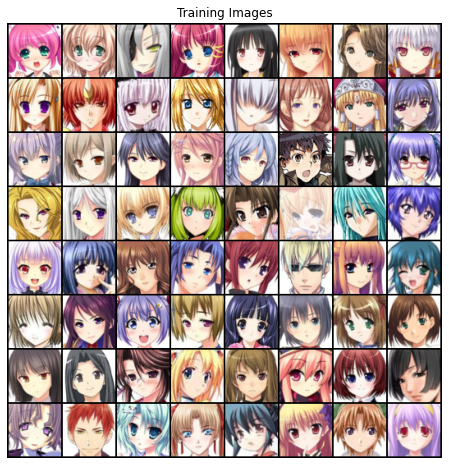
Our dataset is the Anime Face dataset, which contains a bit more than 63’000 colored anime faces. The dataset is donwloaded from the Kaggle website and stored in a local directory. This implementation follows closely the official PyTorch example with minor modifications. The most important parameters are below and require little explanation. The learning rate and the beta1 parameters are as described in the DCGAN paper, and the image size is set to 64, so we will generate $64 \times 64$ color images.
# batch size during training
batch_size = 128

# all images will be resized to this size using a transformer.
image_size = 64

# number of channels in the training images. For color images this is 3
num_channels = 3

# size of z latent vector (i.e. size of generator input)
num_latent = 100

# size of feature maps in generator
num_gen_features = 64

# size of feature maps in discriminator
num_disc_features = 64

# number of training epochs
num_epochs = 50

# learning rate for optimizers
lr = 0.0002

# beta1 hyperparam for Adam optimizers
beta1 = 0.5
Torch transformers are very easy to set up: we resize all the images to be the size we want, we center them, transform to tensor and make sure they are normalized in the $[-1, 1]$ range by subtracting the estimated mean of 0.5 and dividing by the estimated standard deviation of 0.5.
transform = transforms.Compose([transforms.Resize(image_size),
                                transforms.CenterCrop(image_size),
                                transforms.ToTensor(),
                                transforms.Normalize((0.5, 0.5, 0.5), (0.5, 0.5, 0.5))])
datadir = './data'
dataset = datasets.ImageFolder(root=datadir, transform=transform)
print(f"Found {len(dataset)} images in directory {datadir}.")

# Create the dataloader on the dataset
dataloader = torch.utils.data.DataLoader(dataset, batch_size=batch_size, shuffle=True)

device = torch.device("cuda:0") if torch.cuda.is_available() else "cpu"
Found 63565 images in directory ./data.
We can visualize a few images to understand what they look like. Since Torch images have the channels as first dimension, we need to rearrange them before calling plt.imshow().
real_batch = next(iter(dataloader))
plt.figure(figsize=(8, 8))
plt.axis("off")
plt.title("Training Images")
sample = vutils.make_grid(real_batch[0].to(device)[:64], padding=2, normalize=True).cpu()
plt.imshow(np.transpose(sample, (1, 2, 0)));
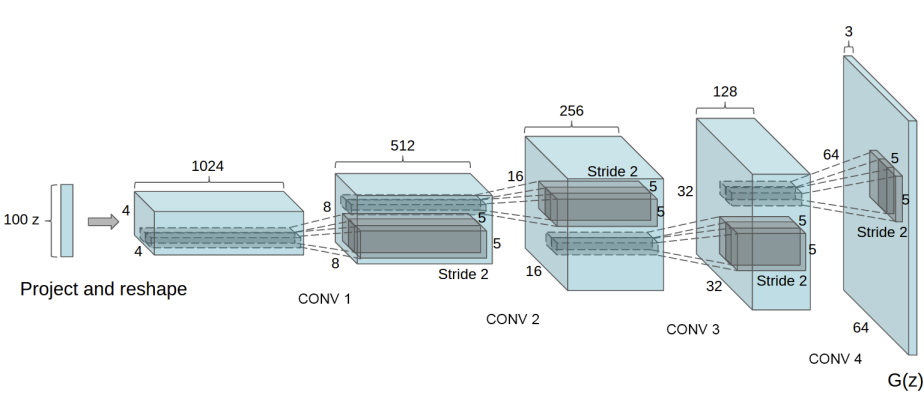
This is the generator class. Transpose convolutions are used to increase the image resolution, while the last layer has a tanh unit as the outputs should be in the $[-1, 1]$ range. The final dimensions are $3 \times 64 \times 64$, where 3 is the number of channels as we want color images, and the images are squared with 64 pixels on each side. The image below is from the paper and shows the generator network.
class Generator(nn.Module):

    def __init__(self, num_latent, num_gen_features, num_channels):
        super().__init__()
        self.main = nn.Sequential(
            # input is noise, going into a convolution
            # Transpose 2D conv layer 1.
            nn.ConvTranspose2d(num_latent, num_gen_features * 8, 4, 1, 0, bias=False),
            nn.BatchNorm2d(num_gen_features * 8),
            nn.ReLU(True),
            # Resulting state size - (num_gen_features*8) x 4 x 4 i.e. if num_gen_features= 64 the size is 512 maps of 4x4

            # Transpose 2D conv layer 2.
            nn.ConvTranspose2d(num_gen_features * 8, num_gen_features * 4, 4, 2, 1, bias=False),
            nn.BatchNorm2d(num_gen_features * 4),
            nn.ReLU(True),
            # Resulting state size -(num_gen_features*4) x 8 x 8 i.e 8x8 maps

            # Transpose 2D conv layer 3.
            nn.ConvTranspose2d(num_gen_features * 4, num_gen_features * 2, 4, 2, 1, bias=False),
            nn.BatchNorm2d(num_gen_features * 2),
            nn.ReLU(True),
            # Resulting state size. (num_gen_features*2) x 16 x 16

            # Transpose 2D conv layer 4.
            nn.ConvTranspose2d(num_gen_features * 2, num_gen_features, 4, 2, 1, bias=False),
            nn.BatchNorm2d(num_gen_features),
            nn.ReLU(True),
            # Resulting state size. (num_gen_features) x 32 x 32

            # Final Transpose 2D conv layer 5 to generate final image.
            nn.ConvTranspose2d(num_gen_features, num_channels, 4, 2, 1, bias=False),

            # Tanh activation to get final normalized image
            nn.Tanh()
            # Resulting state size. (num_channels) x 64 x 64
        )

    def forward(self, x):
        "Takes the noise vector and generates an image"
        return self.main(x)
In the paper, the authors suggest to initialize the weights using a normal distribution with mean 0 and standard deviation of 0.02.
def weights_init(m):
    classname = m.__class__.__name__
    if classname.find('Conv') != -1:
        nn.init.normal_(m.weight.data, 0.0, 0.02)
    elif classname.find('BatchNorm') != -1:
        nn.init.normal_(m.weight.data, 1.0, 0.02)
        nn.init.constant_(m.bias.data, 0)
gen = Generator(num_latent, num_gen_features, num_channels).to(device)
gen.apply(weights_init)
gen
Generator(
  (main): Sequential(
    (0): ConvTranspose2d(100, 512, kernel_size=(4, 4), stride=(1, 1), bias=False)
    (1): BatchNorm2d(512, eps=1e-05, momentum=0.1, affine=True, track_running_stats=True)
    (2): ReLU(inplace=True)
    (3): ConvTranspose2d(512, 256, kernel_size=(4, 4), stride=(2, 2), padding=(1, 1), bias=False)
    (4): BatchNorm2d(256, eps=1e-05, momentum=0.1, affine=True, track_running_stats=True)
    (5): ReLU(inplace=True)
    (6): ConvTranspose2d(256, 128, kernel_size=(4, 4), stride=(2, 2), padding=(1, 1), bias=False)
    (7): BatchNorm2d(128, eps=1e-05, momentum=0.1, affine=True, track_running_stats=True)
    (8): ReLU(inplace=True)
    (9): ConvTranspose2d(128, 64, kernel_size=(4, 4), stride=(2, 2), padding=(1, 1), bias=False)
    (10): BatchNorm2d(64, eps=1e-05, momentum=0.1, affine=True, track_running_stats=True)
    (11): ReLU(inplace=True)
    (12): ConvTranspose2d(64, 3, kernel_size=(4, 4), stride=(2, 2), padding=(1, 1), bias=False)
    (13): Tanh()
  )
)
And this is the discriminator class. The job of the discriminator is a bit easier since it outputs one single number and not an entire image. This number is the probability that the input image is real or fake, so it is in fact a binary classifier. For this reason, Last layer is the sigmoid unit as outputs should be in the $[0, 1]$ range.
class Discriminator(nn.Module):

    def __init__(self, num_disc_features, num_channels):
        super().__init__()
        self.main = nn.Sequential(
            # input is (num_channels) x 64 x 64
            # Conv layer 1:
            nn.Conv2d(num_channels, num_disc_features, 4, 2, 1, bias=False),
            nn.LeakyReLU(0.2, inplace=True),
            # Resulting state size. (num_disc_features) x 32 x 32

            # Conv layer 2:
            nn.Conv2d(num_disc_features, num_disc_features * 2, 4, 2, 1, bias=False),
            nn.BatchNorm2d(num_disc_features * 2),
            nn.LeakyReLU(0.2, inplace=True),
            # Resulting state size. (num_disc_features*2) x 16 x 16

            # Conv layer 3:
            nn.Conv2d(num_disc_features * 2, num_disc_features * 4, 4, 2, 1, bias=False),
            nn.BatchNorm2d(num_disc_features * 4),
            nn.LeakyReLU(0.2, inplace=True),
            # Resulting state size. (num_disc_features*4) x 8 x 8

            # Conv layer 4:
            nn.Conv2d(num_disc_features * 4, num_disc_features * 8, 4, 2, 1, bias=False),
            nn.BatchNorm2d(num_disc_features * 8),
            nn.LeakyReLU(0.2, inplace=True),
            # Resulting state size. (num_disc_features*8) x 4 x 4

            #Conv layer 5:
            nn.Conv2d(num_disc_features * 8, 1, 4, 1, 0, bias=False),

            # Sigmoid Activation:
            nn.Sigmoid()
        )

    def forward(self, input):
        '''Takes as input an image'''
        return self.main(input)
disc = Discriminator(num_disc_features, num_channels).to(device)
disc.apply(weights_init)
disc
Discriminator(
  (main): Sequential(
    (0): Conv2d(3, 64, kernel_size=(4, 4), stride=(2, 2), padding=(1, 1), bias=False)
    (1): LeakyReLU(negative_slope=0.2, inplace=True)
    (2): Conv2d(64, 128, kernel_size=(4, 4), stride=(2, 2), padding=(1, 1), bias=False)
    (3): BatchNorm2d(128, eps=1e-05, momentum=0.1, affine=True, track_running_stats=True)
    (4): LeakyReLU(negative_slope=0.2, inplace=True)
    (5): Conv2d(128, 256, kernel_size=(4, 4), stride=(2, 2), padding=(1, 1), bias=False)
    (6): BatchNorm2d(256, eps=1e-05, momentum=0.1, affine=True, track_running_stats=True)
    (7): LeakyReLU(negative_slope=0.2, inplace=True)
    (8): Conv2d(256, 512, kernel_size=(4, 4), stride=(2, 2), padding=(1, 1), bias=False)
    (9): BatchNorm2d(512, eps=1e-05, momentum=0.1, affine=True, track_running_stats=True)
    (10): LeakyReLU(negative_slope=0.2, inplace=True)
    (11): Conv2d(512, 1, kernel_size=(4, 4), stride=(1, 1), bias=False)
    (12): Sigmoid()
  )
)
As discussed above, we use the BCE loss function. BCE is designed for classification tasks where there are two outcomes (in our case, real and fake). The loss function is
\[J(\vartheta) = -\frac{1}{m} \sum_{i=1}^m \left[ y^{(i)} \log h(x^{(i)}; \vartheta) + (1 - y^{(i)}) \log \left( 1 - h(x^{(i)}; \vartheta) \right) \right],\]where $x^{(i)}$ are the features passed, $y^{(i)}$ is the label, $h(x^{(i)}; \vartheta)$ the prediction made by the model, and $\vartheta$ the parameters of the model. The summation symbol is to compute the average across the minibatch.
The formula looks complicated but it is quite simple. Let’s take a look at the first term, which is the product of the true label times the logarithm of the prediction, which is a probability between 0 and 1. If the true prediction is zero this term is always zero; if the true predicton is one, then this term is small if the prediction is close to one, or very negative if the prediction is close to zero. The same holds true for the other term, mutatis mutandis. The minus sign is used to have a loss function that is smaller when labels and predictions are similar.
criterion = nn.BCELoss()
We define two variables for real and fake labels to make the code easier to read.
REAL_LABEL = 1.0
FAKE_LABEL = 0.0
We need to create two optimizers, one for the generator and a second one for the discriminator.
disc_opt = optim.Adam(disc.parameters(), lr=lr, betas=(beta1, 0.999))
gen_opt = optim.Adam(gen.parameters(), lr=lr, betas=(beta1, 0.999))
To visualize the progress of the generator, we define a noise vector that we keep fixed and we use to generate images at each step of the optimization.
fixed_noise = torch.randn(64, num_latent, 1, 1, device=device)
Training Loop
img_list = []
gen_losses = []
disc_losses = []
iters = 0

for epoch in range(num_epochs):
    for i, data in enumerate(dataloader, 0):
        data = data[0].to(device)
        data_size = data.size(0)

        # ----------------------- #
        # train the discriminator #
        # ----------------------- #

        disc.zero_grad()

        # train using real data
        label = torch.full((data_size,), REAL_LABEL, device=device)
        # forward pass real batch through D
        output = disc(data).view(-1)
        # calculate loss on real batch
        disc_loss_real = criterion(output, label)
        disc_loss_real.backward()
        D_x = output.mean().item()

        # train using fake images from a noise vector given to the generator
        noise = torch.randn(data_size, num_latent, 1, 1, device=device)
        fake = gen(noise)
        label.fill_(FAKE_LABEL)
        output = disc(fake.detach()).view(-1)
        # calculate loss on fake batch
        disc_loss_fake = criterion(output, label)
        # we accumulate the gradients from fake data over those already computed with real data
        disc_loss_fake.backward()
        # update the discriminator
        disc_opt.step()

        # for output, add the gradients from the all-real and all-fake batches
        disc_loss = disc_loss_real + disc_loss_fake
        D_G_z1 = output.mean().item()

        # ------------------- #
        # train the generator #
        # ------------------- #

        gen.zero_grad()
        # as described in the original paper (Section 3), it is better to mark the images as real
        # to get better gradients
        label.fill_(REAL_LABEL)
        # we reuse the same fake images just created, however since we just updated
        # the discriminator, we perform another forward pass of all-fake batch through it
        output = disc(fake).view(-1)
        gen_loss = criterion(output, label)
        gen_loss.backward()
        gen_opt.step()

        # for output
        D_G_z2 = output.mean().item()

        # Output training stats every 50th Iteration in an epoch
        if (i + 1) == len(dataloader):
            print('[%2d/%2d][%3d/%3d]\tLoss_D: %.4f\tLoss_G: %.4f\tD(x): %.4f\tD(G(z)): %.4f => %.4f'
                  % (epoch + 1, num_epochs, i + 1, len(dataloader),
                     disc_loss.item(), gen_loss.item(), D_x, D_G_z1, D_G_z2))

        # Save Losses for plotting later
        gen_losses.append(gen_loss.item())
        disc_losses.append(disc_loss.item())

        # Check how the generator is doing by saving G's output on a fixed_noise vector at the end of each epoch
        if (i + 1) == len(dataloader):
            with torch.no_grad():
                fake = gen(fixed_noise).detach().cpu()
            img_list.append(vutils.make_grid(fake, padding=2, normalize=True))

        iters += 1
[ 1/50][497/497]	Loss_D: 0.4779	Loss_G: 5.5335	D(x): 0.9130	D(G(z)): 0.2928 / 0.0052
[ 2/50][497/497]	Loss_D: 0.3700	Loss_G: 4.7839	D(x): 0.9135	D(G(z)): 0.2166 / 0.0121
[ 3/50][497/497]	Loss_D: 0.2283	Loss_G: 3.9693	D(x): 0.9169	D(G(z)): 0.1211 / 0.0243
[ 4/50][497/497]	Loss_D: 0.8369	Loss_G: 4.9066	D(x): 0.5323	D(G(z)): 0.0010 / 0.0128
[ 5/50][497/497]	Loss_D: 0.2990	Loss_G: 4.5389	D(x): 0.8759	D(G(z)): 0.1324 / 0.0146
[ 6/50][497/497]	Loss_D: 1.4558	Loss_G: 12.3168	D(x): 0.9995	D(G(z)): 0.6729 / 0.0000
[ 7/50][497/497]	Loss_D: 0.1700	Loss_G: 4.6430	D(x): 0.9159	D(G(z)): 0.0667 / 0.0168
[ 8/50][497/497]	Loss_D: 0.1882	Loss_G: 3.7391	D(x): 0.8755	D(G(z)): 0.0393 / 0.0391
[ 9/50][497/497]	Loss_D: 0.3500	Loss_G: 6.4754	D(x): 0.9580	D(G(z)): 0.2277 / 0.0027
[10/50][497/497]	Loss_D: 0.0639	Loss_G: 5.3468	D(x): 0.9700	D(G(z)): 0.0314 / 0.0083
[11/50][497/497]	Loss_D: 0.4529	Loss_G: 3.4082	D(x): 0.7077	D(G(z)): 0.0124 / 0.0557
[12/50][497/497]	Loss_D: 0.2310	Loss_G: 6.7570	D(x): 0.9799	D(G(z)): 0.1720 / 0.0019
[13/50][497/497]	Loss_D: 0.7363	Loss_G: 3.2846	D(x): 0.5680	D(G(z)): 0.0037 / 0.0806
[14/50][497/497]	Loss_D: 0.0936	Loss_G: 4.1996	D(x): 0.9259	D(G(z)): 0.0108 / 0.0257
[15/50][497/497]	Loss_D: 0.3975	Loss_G: 4.7041	D(x): 0.8820	D(G(z)): 0.1953 / 0.0139
[16/50][497/497]	Loss_D: 0.1048	Loss_G: 3.7161	D(x): 0.9252	D(G(z)): 0.0215 / 0.0476
[17/50][497/497]	Loss_D: 0.2865	Loss_G: 4.8236	D(x): 0.9434	D(G(z)): 0.1826 / 0.0120
[18/50][497/497]	Loss_D: 0.2049	Loss_G: 5.7258	D(x): 0.9879	D(G(z)): 0.1613 / 0.0046
[19/50][497/497]	Loss_D: 0.1488	Loss_G: 4.6520	D(x): 0.9574	D(G(z)): 0.0902 / 0.0152
[20/50][497/497]	Loss_D: 0.1350	Loss_G: 4.5557	D(x): 0.9586	D(G(z)): 0.0808 / 0.0151
[21/50][497/497]	Loss_D: 0.2963	Loss_G: 5.1431	D(x): 0.9196	D(G(z)): 0.1629 / 0.0103
[22/50][497/497]	Loss_D: 0.1232	Loss_G: 5.4050	D(x): 0.9925	D(G(z)): 0.0962 / 0.0067
[23/50][497/497]	Loss_D: 0.6058	Loss_G: 8.0698	D(x): 0.9985	D(G(z)): 0.3791 / 0.0005
[24/50][497/497]	Loss_D: 0.1115	Loss_G: 6.0990	D(x): 0.9822	D(G(z)): 0.0816 / 0.0035
[25/50][497/497]	Loss_D: 0.6234	Loss_G: 5.2236	D(x): 0.9582	D(G(z)): 0.3716 / 0.0085
[26/50][497/497]	Loss_D: 0.1634	Loss_G: 4.9527	D(x): 0.8859	D(G(z)): 0.0240 / 0.0146
[27/50][497/497]	Loss_D: 0.1378	Loss_G: 3.0970	D(x): 0.9092	D(G(z)): 0.0298 / 0.0711
[28/50][497/497]	Loss_D: 0.2245	Loss_G: 4.1251	D(x): 0.9765	D(G(z)): 0.1611 / 0.0228
[29/50][497/497]	Loss_D: 0.0693	Loss_G: 4.5140	D(x): 0.9537	D(G(z)): 0.0197 / 0.0167
[30/50][497/497]	Loss_D: 0.0578	Loss_G: 5.0501	D(x): 0.9695	D(G(z)): 0.0245 / 0.0120
[31/50][497/497]	Loss_D: 0.1976	Loss_G: 5.1063	D(x): 0.8784	D(G(z)): 0.0390 / 0.0172
[32/50][497/497]	Loss_D: 0.2303	Loss_G: 8.8036	D(x): 0.9904	D(G(z)): 0.1759 / 0.0002
[33/50][497/497]	Loss_D: 0.0540	Loss_G: 4.8158	D(x): 0.9751	D(G(z)): 0.0268 / 0.0141
[34/50][497/497]	Loss_D: 0.4928	Loss_G: 1.6454	D(x): 0.6852	D(G(z)): 0.0139 / 0.2943
[35/50][497/497]	Loss_D: 0.0911	Loss_G: 4.9199	D(x): 0.9738	D(G(z)): 0.0566 / 0.0114
[36/50][497/497]	Loss_D: 0.1957	Loss_G: 4.2353	D(x): 0.8778	D(G(z)): 0.0273 / 0.0294
[37/50][497/497]	Loss_D: 0.0431	Loss_G: 5.3940	D(x): 0.9839	D(G(z)): 0.0257 / 0.0073
[38/50][497/497]	Loss_D: 0.0567	Loss_G: 5.1527	D(x): 0.9721	D(G(z)): 0.0264 / 0.0107
[39/50][497/497]	Loss_D: 0.0576	Loss_G: 4.9289	D(x): 0.9872	D(G(z)): 0.0422 / 0.0116
[40/50][497/497]	Loss_D: 0.3995	Loss_G: 4.3143	D(x): 0.8548	D(G(z)): 0.1454 / 0.0230
[41/50][497/497]	Loss_D: 0.0551	Loss_G: 5.2280	D(x): 0.9797	D(G(z)): 0.0318 / 0.0097
[42/50][497/497]	Loss_D: 0.1024	Loss_G: 4.4772	D(x): 0.9493	D(G(z)): 0.0421 / 0.0191
[43/50][497/497]	Loss_D: 0.0974	Loss_G: 5.4068	D(x): 0.9482	D(G(z)): 0.0382 / 0.0101
[44/50][497/497]	Loss_D: 0.1233	Loss_G: 4.9374	D(x): 0.9492	D(G(z)): 0.0575 / 0.0143
[45/50][497/497]	Loss_D: 0.0417	Loss_G: 5.4731	D(x): 0.9869	D(G(z)): 0.0272 / 0.0077
[46/50][497/497]	Loss_D: 0.1162	Loss_G: 4.8060	D(x): 0.9376	D(G(z)): 0.0442 / 0.0148
[47/50][497/497]	Loss_D: 0.0205	Loss_G: 5.9650	D(x): 0.9905	D(G(z)): 0.0108 / 0.0054
[48/50][497/497]	Loss_D: 0.0324	Loss_G: 5.7304	D(x): 0.9808	D(G(z)): 0.0125 / 0.0062
[49/50][497/497]	Loss_D: 0.1013	Loss_G: 5.8835	D(x): 0.9709	D(G(z)): 0.0570 / 0.0053
[50/50][497/497]	Loss_D: 0.0487	Loss_G: 5.9634	D(x): 0.9886	D(G(z)): 0.0347 / 0.0053
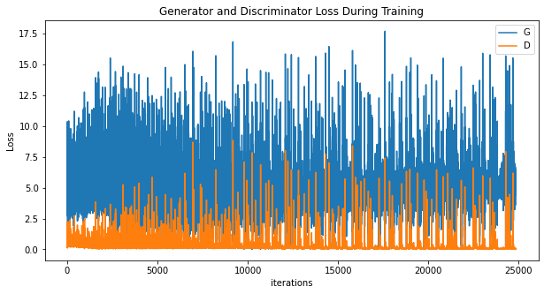
plt.figure(figsize=(10,5))
plt.title("Generator and Discriminator Loss During Training")
plt.plot(gen_losses,label="G")
plt.plot(disc_losses,label="D")
plt.xlabel("iterations")
plt.ylabel("Loss")
plt.legend()
plt.show()
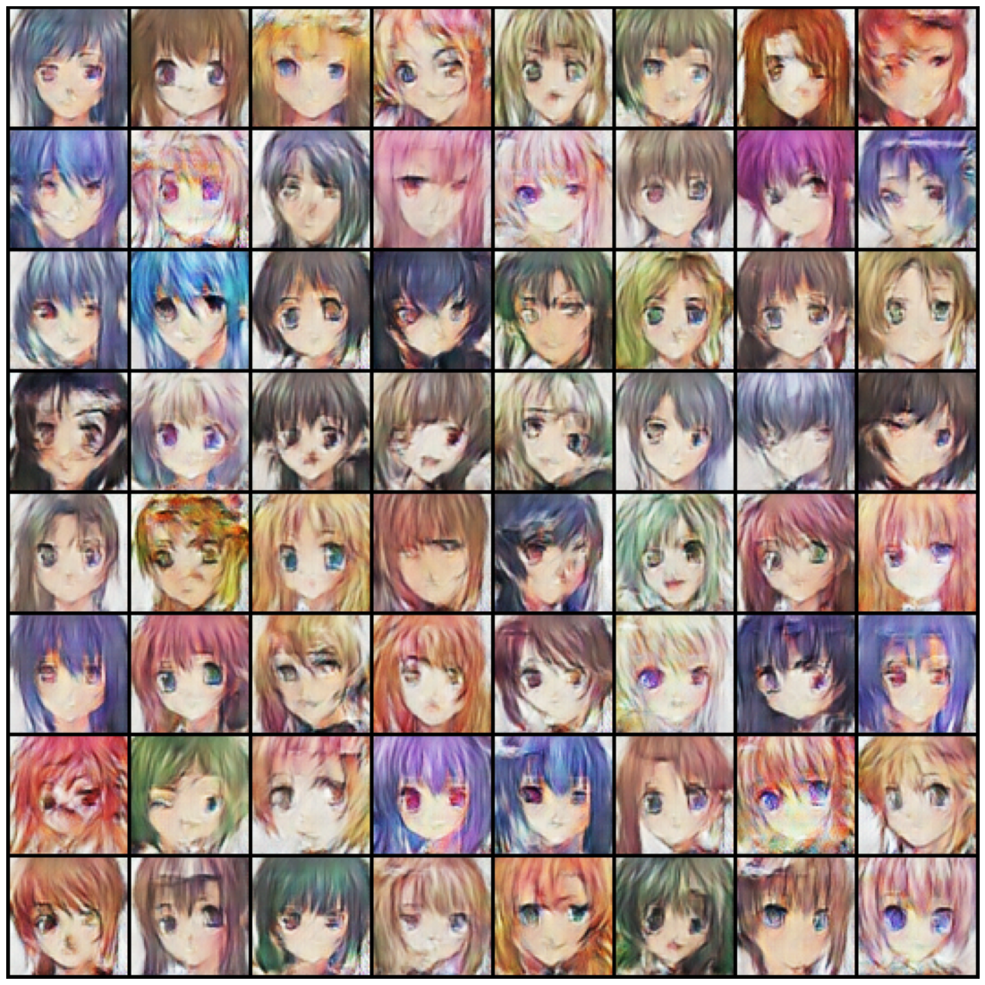
Images generated after 10 epochs – they look ok, but are still quite blurry and often miss some features.
plt.figure(figsize=(20, 20))
plt.axis('off')
plt.imshow(np.transpose(img_list[10], (1, 2, 0)), animated=True);
After 20 epochs results are better:
plt.figure(figsize=(20, 20))
plt.axis('off')
plt.imshow(np.transpose(img_list[20], (1, 2, 0)), animated=True);
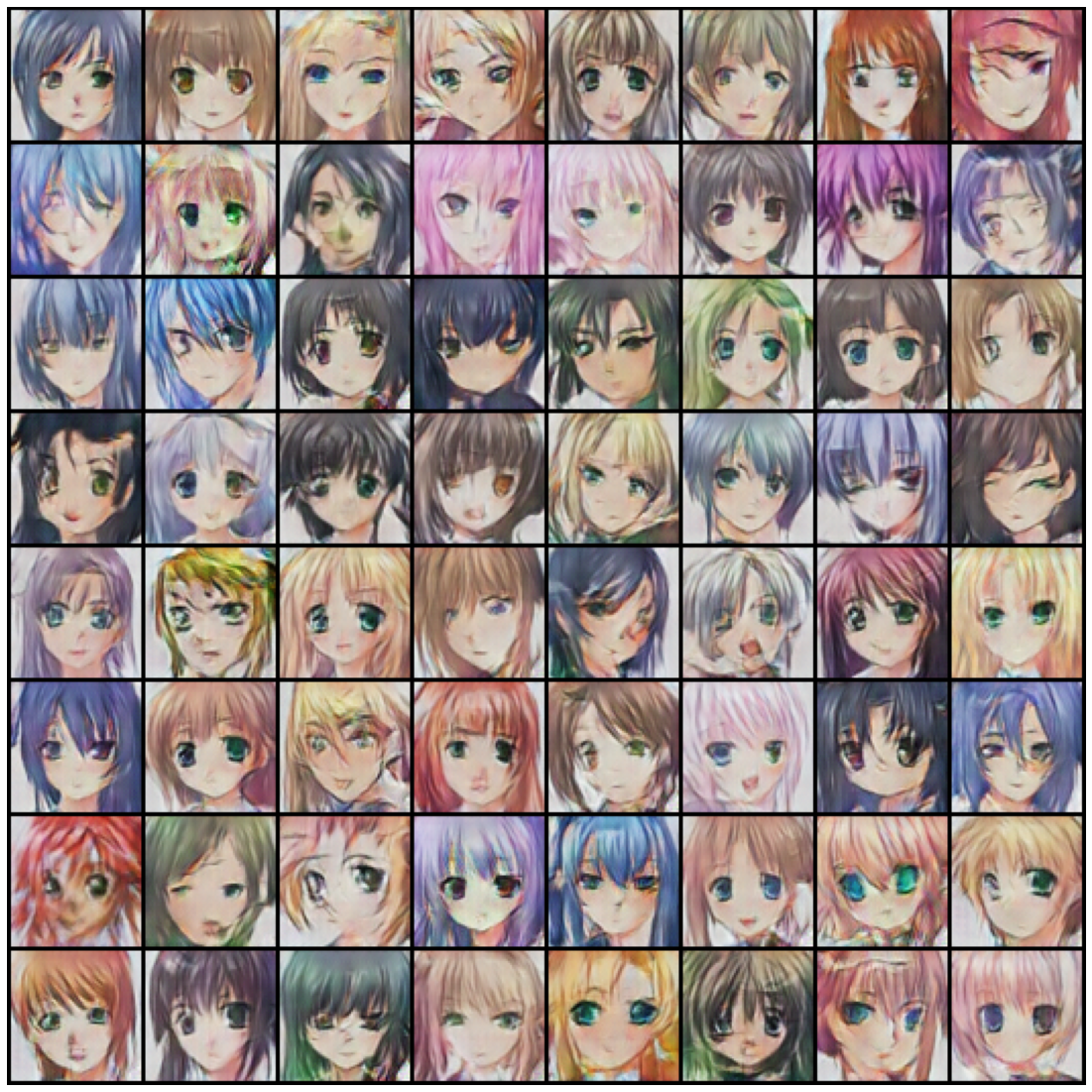
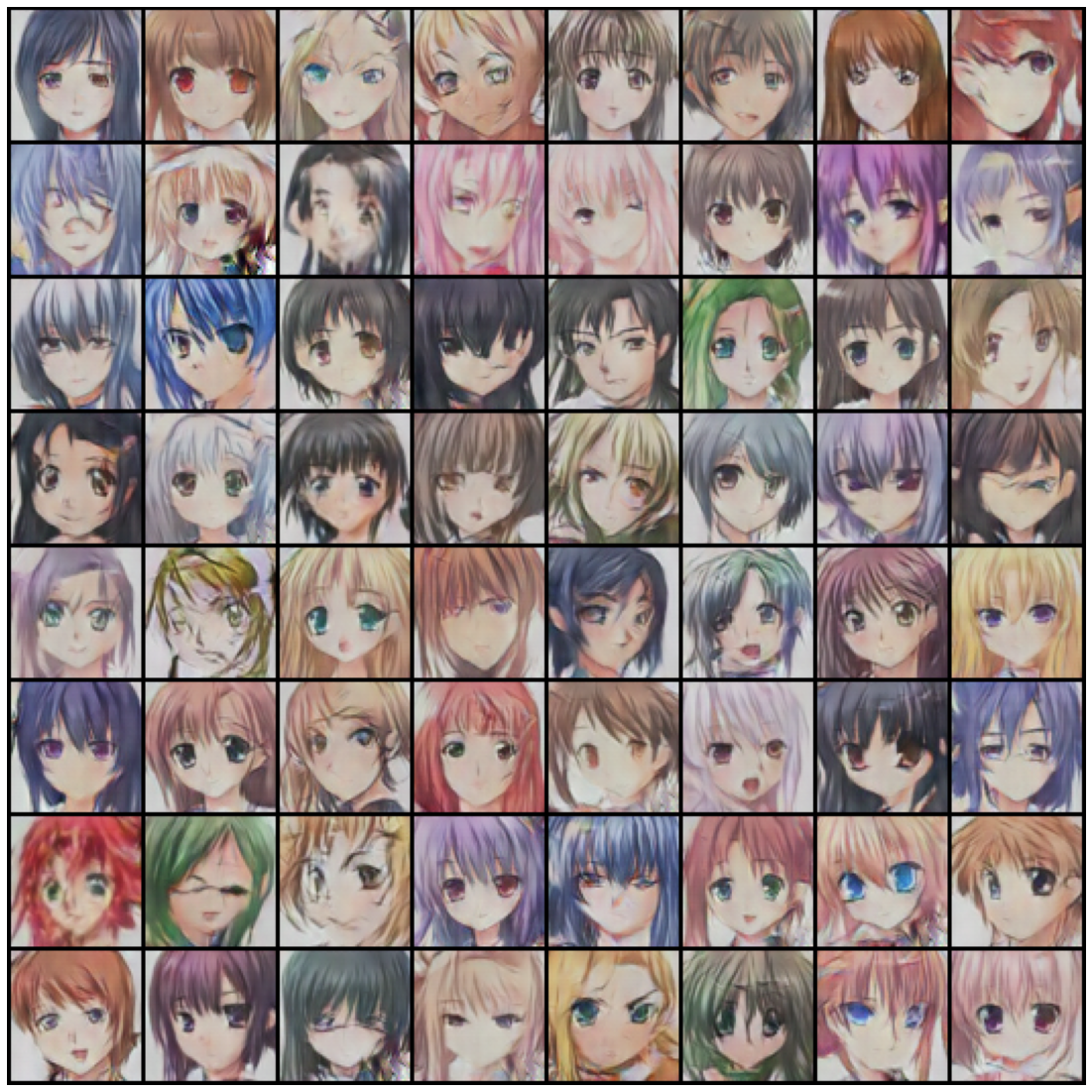
And finally this is after 50 epochs. Not all images are good – some miss the mouth, for example, or look at the one on the right of the first row which seems to have one eye only, but overall they are good and relatively sharp.
plt.figure(figsize=(20, 20))
plt.axis('off')
plt.imshow(np.transpose(img_list[-1], (1, 2, 0)), animated=True);