In this article we look at bagging, or bootstrap aggregating, a powerful and intuitive ensemble technique that reduces variance, enhances robustness, and improves overall predictive accuracy. This technique is particularly effective for high-variance models, such as deep decision trees, where it forms the backbone of popular algorithms like Random Forest, but it can be used with any type of method. Bagging is a special case of the ensemble averaging approach.
Instead of relying on a single model, bagging constructs an ensemble of models, each trained on a randomly sampled subset of the training data. The idea is to average the predictions of these models (for regression) or use majority voting (for classification).
Bagging does not reduce bias; it only reduces variance. It is most effective when the base models are high-variance, low-bias estimators (e.g., deep decision trees).
import numpy as np
import pandas as pd
import matplotlib.pyplot as plt
from sklearn.model_selection import train_test_split, cross_val_score
from sklearn.tree import DecisionTreeClassifier
from sklearn.ensemble import BaggingClassifier
from sklearn.metrics import accuracy_score, classification_report, confusion_matrix, f1_score
from sklearn.preprocessing import LabelEncoder
import seaborn as sns
We will use a dataset that contains the income of several people around the world. The data is a bit old since it refers to 1994 and has 32’561 rows.
url = "https://archive.ics.uci.edu/ml/machine-learning-databases/adult/adult.data"
column_names = [
    'age', 'workclass', 'fnlwgt', 'education', 'education-num',
    'marital-status', 'occupation', 'relationship', 'race', 'sex',
    'capital-gain', 'capital-loss', 'hours-per-week', 'native-country', 'income',
]

df = pd.read_csv(url, names=column_names, sep=',\\s*', engine='python', na_values='?')
print(f"The dataset contains {df.shape[0]} rows and {df.shape[1]} columns.\n")
df.sample(5)
The dataset contains 32561 rows and 15 columns.
| age | workclass | fnlwgt | education | education-num | marital-status | occupation | relationship | race | sex | capital-gain | capital-loss | hours-per-week | native-country | income | |
|---|---|---|---|---|---|---|---|---|---|---|---|---|---|---|---|
| 26934 | 24 | Local-gov | 452640 | Some-college | 10 | Never-married | Tech-support | Not-in-family | White | Male | 14344 | 0 | 50 | United-States | >50K |
| 15798 | 40 | Private | 209833 | HS-grad | 9 | Never-married | Craft-repair | Not-in-family | White | Male | 0 | 0 | 40 | United-States | <=50K |
| 29713 | 19 | Local-gov | 243960 | Some-college | 10 | Never-married | Sales | Own-child | White | Female | 0 | 0 | 16 | United-States | <=50K |
| 16011 | 39 | Private | 186420 | HS-grad | 9 | Divorced | Adm-clerical | Not-in-family | White | Female | 0 | 0 | 40 | United-States | <=50K |
| 30899 | 30 | Federal-gov | 127610 | Bachelors | 13 | Never-married | Adm-clerical | Not-in-family | White | Female | 0 | 0 | 35 | United-States | <=50K |
The meaning of the columns is the following:
- age: discrete (from 17 to 90)
- workclass (private, federal-government, etc): nominal (9 categories)
- fnlwgt: the final weight (the number of people the census believes the entry represents): discrete
- education (the highest level of education obtained): ordinal (16 categories)
- education-num (the number of years of education): discrete (from 1 to 16)
- marital-status: nominal (7 categories)
- occupation (transport-moving, craft-repair, etc): nominal (15 categories)
- relationship in family (unmarried, not in the family, etc): nominal (6 categories)
- race: nominal (5 categories)
- sex: nominal (2 categories)
- capital-gain: continuous
- capital-loss: continuous
- hours-per-week (hours worked per week(): discrete (from 1 to 99)
- native-country: nominal (42 countries)
- income (whether or not an individual makes more than $50,000 annually): boolean (≤$50k, >$50k)
df = df.dropna()
print(f"# rows after removing missing values: {len(df)}")
# rows after removing missing values: 30162
df.describe(include='all').T
| count | unique | top | freq | mean | std | min | 25% | 50% | 75% | max | |
|---|---|---|---|---|---|---|---|---|---|---|---|
| age | 32561.0 | NaN | NaN | NaN | 38.581647 | 13.640433 | 17.0 | 28.0 | 37.0 | 48.0 | 90.0 |
| workclass | 30725 | 8 | Private | 22696 | NaN | NaN | NaN | NaN | NaN | NaN | NaN |
| fnlwgt | 32561.0 | NaN | NaN | NaN | 189778.366512 | 105549.977697 | 12285.0 | 117827.0 | 178356.0 | 237051.0 | 1484705.0 |
| education | 32561 | 16 | HS-grad | 10501 | NaN | NaN | NaN | NaN | NaN | NaN | NaN |
| education-num | 32561.0 | NaN | NaN | NaN | 10.080679 | 2.57272 | 1.0 | 9.0 | 10.0 | 12.0 | 16.0 |
| marital-status | 32561 | 7 | Married-civ-spouse | 14976 | NaN | NaN | NaN | NaN | NaN | NaN | NaN |
| occupation | 30718 | 14 | Prof-specialty | 4140 | NaN | NaN | NaN | NaN | NaN | NaN | NaN |
| relationship | 32561 | 6 | Husband | 13193 | NaN | NaN | NaN | NaN | NaN | NaN | NaN |
| race | 32561 | 5 | White | 27816 | NaN | NaN | NaN | NaN | NaN | NaN | NaN |
| sex | 32561 | 2 | Male | 21790 | NaN | NaN | NaN | NaN | NaN | NaN | NaN |
| capital-gain | 32561.0 | NaN | NaN | NaN | 1077.648844 | 7385.292085 | 0.0 | 0.0 | 0.0 | 0.0 | 99999.0 |
| capital-loss | 32561.0 | NaN | NaN | NaN | 87.30383 | 402.960219 | 0.0 | 0.0 | 0.0 | 0.0 | 4356.0 |
| hours-per-week | 32561.0 | NaN | NaN | NaN | 40.437456 | 12.347429 | 1.0 | 40.0 | 40.0 | 45.0 | 99.0 |
| native-country | 31978 | 41 | United-States | 29170 | NaN | NaN | NaN | NaN | NaN | NaN | NaN |
| income | 32561 | 2 | <=50K | 24720 | NaN | NaN | NaN | NaN | NaN | NaN | NaN |
education_order = [
    'Preschool',
    '1st-4th',
    '5th-6th',
    '7th-8th',
    '9th',
    '10th',
    '11th',
    '12th',
    'HS-grad',
    'Some-college',
    'Assoc-voc',
    'Assoc-acdm',
    'Bachelors',
    'Masters',
    'Prof-school',
    'Doctorate'
]
plt.figure(figsize=(12, 6))
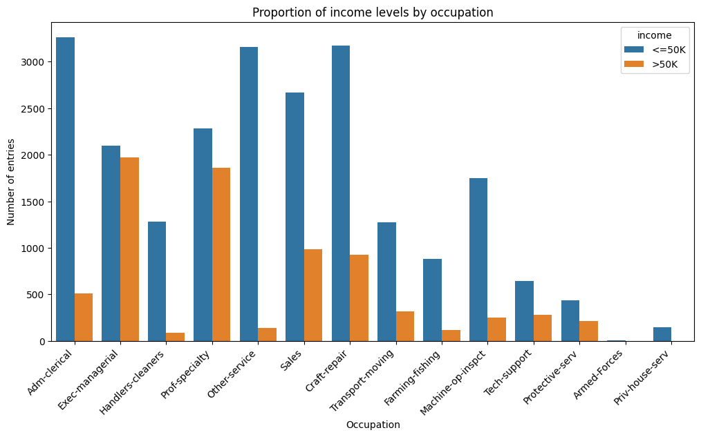
sns.countplot(data=df, x='occupation', hue='income')
plt.title('Proportion of income levels by occupation')
plt.xlabel('Occupation')
plt.ylabel('Number of entries')
plt.xticks(rotation=45, ha='right');
income_proportions = pd.crosstab(df['education'], df['income'], normalize='index')
income_proportions = income_proportions.reset_index()
income_proportions = income_proportions.melt(id_vars='education', var_name='income', value_name='proportion')

# Sort by the education_levels order
income_proportions['education'] = pd.Categorical(income_proportions['education'], categories=education_order, ordered=True)
income_proportions = income_proportions.sort_values('education')

plt.figure(figsize=(12, 6))
sns.barplot(
    data=income_proportions,
    x='education',
    y='proportion',
    hue='income'
)

plt.title('Proportion of income levels by education')
plt.xlabel('Education')
plt.ylabel('Proportion')
plt.xticks(rotation=45, ha='right')
plt.tight_layout()
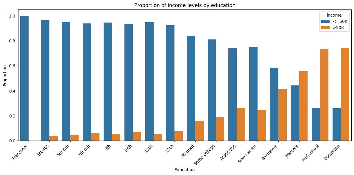
As one would expect, we see from the bar graph that as the education level increase, the proportion of people who earn more than 50k a year also increase. It is interesting to note that only after a master’s degree, the proportion of people earning more than 50k a year, is a majority.
plt.figure(figsize=(12, 6))
sns.histplot(data=df, x='age', hue='sex', bins=20, multiple='dodge', kde=True)
plt.title('Age Distribution', pad=20)
plt.xlabel('Age', labelpad=10)
plt.ylabel('Count', labelpad=10)
plt.tight_layout()
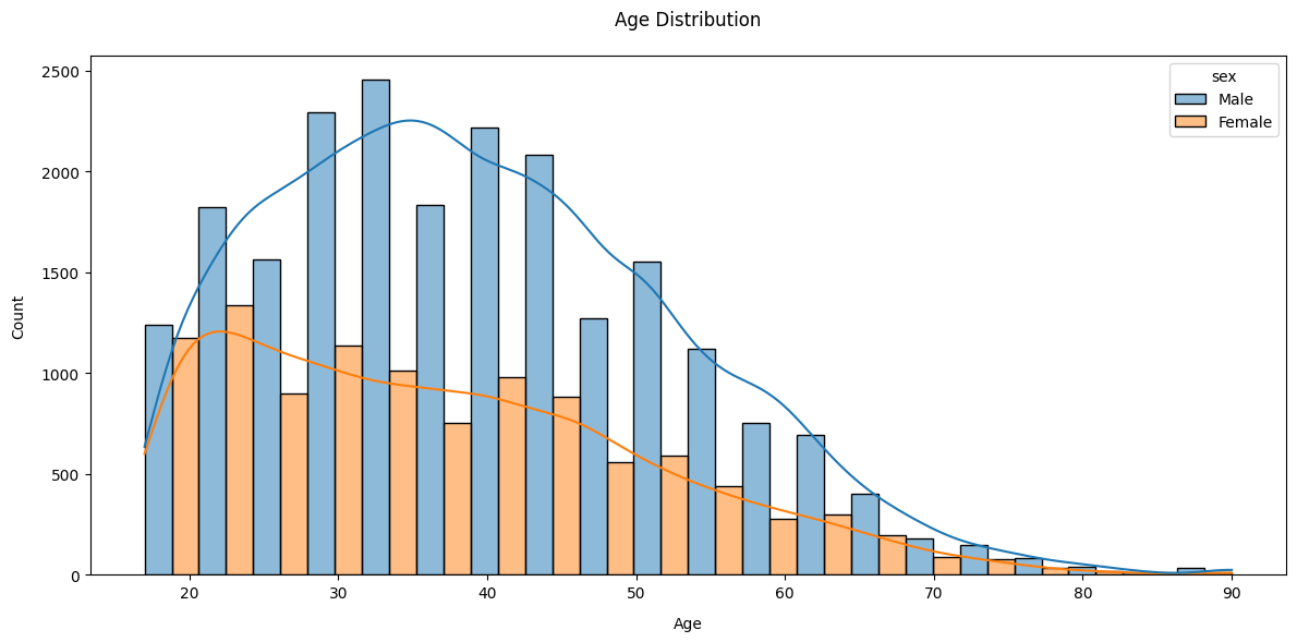
Distribution of income by age is as expected as well, at least for males: it grows with age, peaking around 40, then dicreases. For females it is instead decreasing from the mid-twenties, possibly because of time invested in the family. This is for 1994’s societies, in today’s value the peak would rather be around 50, with less distortion between males and females. Gender disparities are shown clearly in the graph below.
plt.figure(figsize=(10, 6))
sns.countplot(data=df, x='sex', hue='income')
plt.title('Income Distribution by Gender')
plt.xlabel('Sex')
plt.ylabel('Count')
plt.legend(title='Income')
plt.tight_layout()
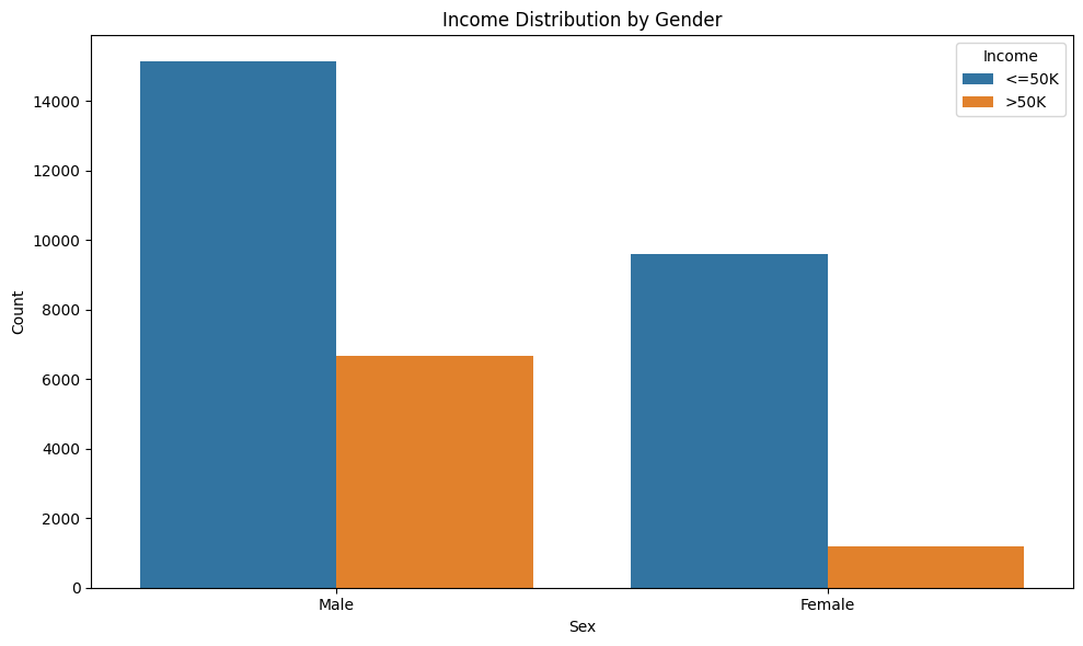
The dataset is slightly unbalanced, with 75% of the entries making less than 50K a year and 25% making more.
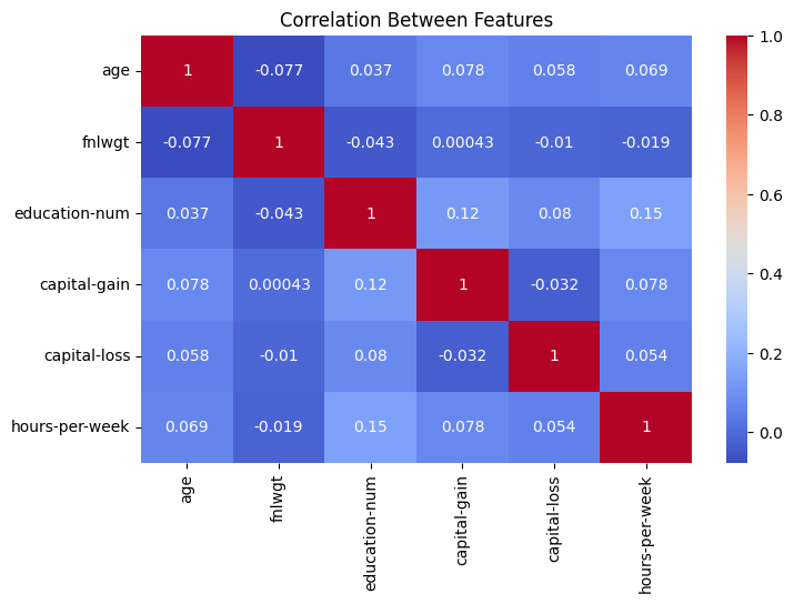
The heatmap with numerical features doesn’t show any strong correlation.
plt.figure(figsize=(8,5))
sns.heatmap(df.select_dtypes(include='number').corr(), annot=True, cmap='coolwarm')
plt.title("Correlation Between Features");
To prepare a model, we select most of the columns. They are both numerical and categorical; the latter are encoded using a one-hot encoding technique.
features_to_use = [
    'age',
    'workclass',
    'education',
    'marital-status',
    'occupation',
    'relationship',
    'race',
    'sex',
    'capital-gain',
    'capital-loss',
    'hours-per-week',
    'native-country',
]

X = df[features_to_use].copy()

label_encoders = {}
categorical_cols = X.select_dtypes(include=['object']).columns
X = pd.get_dummies(X, columns=categorical_cols, drop_first=True)

y = df['income'].copy()
y = (y == '>50K').astype(int)
print(f"# positive entries: {y.mean():.2%}, # negative entries: {(1 - y).mean():.2%}")
print(f"Final number of features (after one-hot encoding): {X.shape[1]}")
# positive entries: 24.08%, # negative entries: 75.92%
Final number of features (after one-hot encoding): 95
X_train, X_test, y_train, y_test = train_test_split(
    X, y, test_size=0.25, random_state=42, stratify=y
)
print(f"# train samples: {len(X_train):,}, # test samples: {len(X_test):,}")
# train samples: 22,621, # test samples: 7,541
single_tree = DecisionTreeClassifier(random_state=42)
single_tree.fit(X_train, y_train)

y_pred_single = single_tree.predict(X_test)
accuracy_single = accuracy_score(y_test, y_pred_single)
f1_single = f1_score(y_test, y_pred_single)

print(f"Test accuracy: {accuracy_single:.4f} ({accuracy_single*100:.2f}%)")
print(f"F1 score: {f1_single:.4f}")

cv_scores_single = cross_val_score(single_tree, X, y, cv=5, scoring='accuracy')
print(f"Cross-validation accuracy: {cv_scores_single.mean():.4f} (+/- {cv_scores_single.std():.4f})")
Test accuracy: 0.8124 (81.24%)
F1 score: 0.6197
Cross-validation accuracy: 0.8184 (+/- 0.0029)
bagging_clf = BaggingClassifier(
    estimator=DecisionTreeClassifier(),
    n_estimators=20,
    max_samples=0.5,
    max_features=1.0,
    bootstrap=True,
    bootstrap_features=True,
    random_state=42,
    n_jobs=-1,
)

bagging_clf.fit(X_train, y_train)

y_pred_bagging = bagging_clf.predict(X_test)
accuracy_bagging = accuracy_score(y_test, y_pred_bagging)
f1_bagging = f1_score(y_test, y_pred_bagging)

print(f"Test accuracy: {accuracy_bagging:.4f} ({accuracy_bagging*100:.2f}%)")
print(f"F1 score: {f1_bagging:.4f}")

cv_scores_bagging = cross_val_score(bagging_clf, X, y, cv=5, scoring='accuracy')
print(f"Cross-validation accuracy: {cv_scores_bagging.mean():.4f} (+/- {cv_scores_bagging.std():.4f})")
Test accuracy: 0.8540 (85.40%)
F1 score: 0.6730
Cross-validation accuracy: 0.8594 (+/- 0.0044)
The result is about 4 percentage point increase in accuracy, both in the test dataset and for the cross-validation, showing the effectiveness of bagging.