The Black-Scholes Model

In this article we cover the Black-Scholes model for modeling a a divideng-paying stock. We will verify the basic property of the model by looking at the realized profit and loss (P/L) of a trader that is short an option and performs delta hedging.

The Python environment is quite simple and requires a few standard packages.

$ python -mv venv venv
$ ./venv/Scripts/activate
$ pip install numpy matplotlib seaborn scipy pandas

We assume that the stock process $S(t)$ follows the dynamics

\[\frac{dS(t)}{S(t)} = (r - q) dt + \sigma dW(t),\]

with $S(0) = S_0$ the initial value, $r$ the deterministic discount factor, $q$ the deterministic dividend yield, and $dW(t)$ a Wiener process. We assume $r$, $q$, and $\sigma$ to be constant values, even if it is easy to extend the results to time-varying (yet deterministic) functions.

from collections import namedtuple
import matplotlib.pylab as plt
import numpy as np
import pandas as pd
from scipy.stats import norm
import seaborn as sns

To keep things simple, we put together all the components of the model into the class Model. All the features of the vanilla contract are in the Vanilla class, where $N$ is the notional of the contract (that is, the number of shares that the client wants to buy or sell), K is the strike, T the expiry, and is_call is a boolean to distinguish put and call options. All times are in fractions of the year, starting from $t=0$.

Model = namedtuple('Model', 'r, q, σ')
Vanilla = namedtuple('Vanilla', 'N, K, T, is_call')

Φ = norm.cdf

It is well-known that the value of a vanilla option at time $t$ is given by the formula

\[C = e^{-r T} \omega \left[ F \, \Phi(ω d_+) - K \, \Phi(ω d_-)) \right]\]

where $K$ is the strike of the option, $\tau = T -t$ is the time to expiry, $F = S(t) e^{(r - q) τ}$ is the forward at time $T$, $\omega$ is 1 for a call and -1 for a put, $\Phi$ the cumulative function of the normal distribution, and

\[\begin{aligned} d_+ & = \frac{\log\frac{F}{K} + \frac{1}{2} σ^2 τ}{σ \sqrt{τ}} \\ d_- & = d_+ - σ * \sqrt{τ}. \end{aligned}\]

def compute_price(t, S_t, r, q, σ, N, K, T, is_call):
    τ = T - t
    ω = 1.0 if is_call else -1.0
    if τ == 0.0:
        return N * max(ω * (S_t - K), 0.0)
    F = S_t * np.exp((r - q) * τ)
    df = np.exp(-r * τ)
    d_plus = (np.log(F / K) + 0.5 * σ**2 * τ) / σ / np.sqrt(τ)
    d_minus = d_plus - σ * np.sqrt(τ)
    return N * ω * df * (F * Φ(ω * d_plus) - K * Φ(ω * d_minus))

To perform delta hedging, a trader needs to build the amount of shares given by the delta of the option, which reads

\[\Delta = ω e^{-r \tau} (F \, Φ(ω d_+) - K \, Φ(ω d_-)).\]

def compute_delta(t, S_t, r, q, σ, N, K, T, is_call):
    τ = T - t
    ω = 1.0 if is_call else -1.0
    if τ == 0.0:
        return 1.0 if ω * (S_t - K) > 0 else 0.0
    F = S_t * np.exp((r - q) * τ)
    d_plus = (np.log(F / K) + 0.5 * σ**2 * τ) / σ / np.sqrt(τ)
    return N * ω * np.exp(-q * τ) * Φ(ω * d_plus)

We need to generate paths that are realization of the Black-Scholes model, as done by the generate_paths() function.

def generate_paths(t_0, S_0, r, q, σ, T, num_paths, num_steps):
    assert T > t_0
    retval = [np.ones((num_paths,)) * S_0]
    X = np.log(retval[0])
    schedule = np.linspace(t_0, T, num_steps + 1)
    W = norm.rvs(size=(num_steps, num_paths))
    t = 0.0
    for i in range(num_steps):
        Δt = schedule[i + 1] - schedule[i]
        t = t + Δt
        sqrt_Δt = np.sqrt(Δt)
        X = X + (r - q - 0.5 * σ**2) * Δt + σ * sqrt_Δt * W[i, :]
        retval.append(np.exp(X))
    return schedule, np.vstack(retval)

The procedure is the following: the trader sells the option and adds the premium to the P/L; then at every time $t$ they purchase $\Delta(t)$ options at spot $S(t)$, costing $S(t) \Delta(t)$, which is the amount we need to subtract to the P/L. At $t + \delta t$ they need to purchase $\Delta(t + \delta t) - \Delta(t)$ options, and so on till expiry. In the interval $[t, t + \delta t)$ the cash accrues the interest $r$, while the shares accrues $q \Delta(t) S(t)$ in dividends. At expiry, the owner of the call will get one share if $S(T) > K$ and will pay $K$, or nothing if $S(T) \le K$; the behavior at expiry for a put option is similar. From the classical theory we would expect a zero P/L over all paths when hedging happens continuously, or a small difference otherwise.

def analyze(t_0, S_0, model, vanilla, num_steps, num_paths):
    ts, paths = generate_paths(t_0, S_0, *model, vanilla.T, num_steps, num_paths)

    pnls = []

    for i in range(paths.shape[1]):
        # compute the PNL over each path
        path = paths[:, i]
        # we are short the option
        premium = compute_price(t_0, S_0, *model, *vanilla)
        cash, shares = premium, 0.0
        # perform hedging on each time interval
        for t, t_plus_Δt, S_t in zip(ts[:-1], ts[1:], path[:-1]):
            Δt = t_plus_Δt - t
            # delta hedge at the beginning of the interval
            new_shares = compute_delta(t, S_t, *model, *vanilla)
            # hedging cost
            cash -= (new_shares - shares) * S_t
            shares = new_shares
            # interests and dividends
            cash += cash * (np.exp(model.r * Δt) - 1) + shares * (np.exp(model.q * Δt) - 1) * S_t

        # at expiry, sell the shares to the client if the option in-the-money
        T, S_T = ts[-1], path[-1]
        if vanilla.is_call and S_T > vanilla.K:
            # sell N shares at value K
            cash += vanilla.K * vanilla.N
            shares -= vanilla.N
        elif not vanilla.is_call and S_T < vanilla.K:
            # buy N shares at value K
            cash -= vanilla.K * vanilla.N
            shares += vanilla.N
        # liquidate all remaining positions, we must have zero shares at the end
        cash += shares * S_T
        pnls.append(cash)

    pnls = np.array(pnls) * np.exp(-model.r * (T -t_0))
    normalized_pnls = pnls / premium
    return normalized_pnls

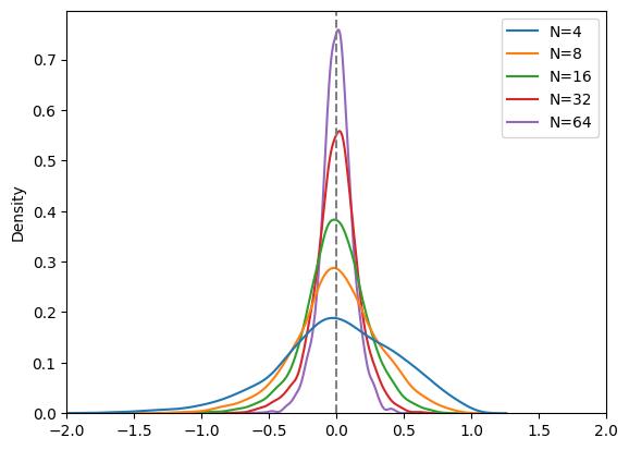
We will analyze two cases: a call option first, then a put option. We take $S_0=100$ and a volatility of 25%. For a fixed number of paths (1,000), we divide the time $[0, T]$ into $n$ interval and perform delta hedging at each point. We would expect to have a P/L distribution that is centered around zero yet a bit scattered (symmetrically), with average errors getting smaller and smaller as $n\rightarrow \infty$. We have plotted the normalized P/L, defined as P/L divided by the option premium.

t_0, S_0 = 0.0, 100.0
model = Model(r=0.0, q=0.2, σ=0.25)
vanilla = Vanilla(N=1.0, K=S_0, T=1.0, is_call=True)

num_paths = 1_000
data = {}
for num_steps in [4, 8, 16, 32, 64]:
    normalized_pnls = analyze(t_0, S_0, model, vanilla, num_paths, num_steps)
    print(f"{num_steps: 2d} steps: E[PNL] = {normalized_pnls.mean():.2f}, V[PNL] = {normalized_pnls.std():.2f}")
    data[f'N={num_steps}'] = normalized_pnls

steps: E[PNL] = 0.06, V[PNL] = 1.15
steps: E[PNL] = 0.06, V[PNL] = 0.84
steps: E[PNL] = 0.04, V[PNL] = 0.58
steps: E[PNL] = 0.01, V[PNL] = 0.42
steps: E[PNL] = -0.00, V[PNL] = 0.30

data = pd.DataFrame(data)
sns.kdeplot(data)
plt.xlim(-2, 2)
plt.axvline(x=0, linestyle='dashed', color='grey');

png

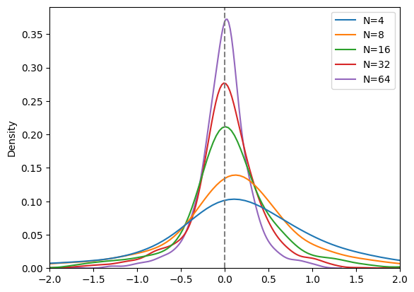
t_0, S_0 = 0.0, 100.0
model = Model(r=0.05, q=0.03, σ=0.25)
vanilla = Vanilla(N=1.0, K=S_0, T=1.0, is_call=False)

num_paths = 4_000
data = {}
for num_steps in [4, 8, 16, 32, 64]:
    normalized_pnls = analyze(t_0, S_0, model, vanilla, num_paths, num_steps)
    print(f"{num_steps: 2d} steps: E[PNL] = {normalized_pnls.mean():.2f}, V[PNL] = {normalized_pnls.std():.2f}")
    data[f'N={num_steps}'] = normalized_pnls

steps: E[PNL] = 0.00, V[PNL] = 0.46
steps: E[PNL] = -0.00, V[PNL] = 0.32
steps: E[PNL] = -0.01, V[PNL] = 0.24
steps: E[PNL] = -0.00, V[PNL] = 0.17
steps: E[PNL] = 0.00, V[PNL] = 0.12

data = pd.DataFrame(data)
sns.kdeplot(data)
plt.xlim(-2, 2)
plt.axvline(x=0, linestyle='dashed', color='grey');

png