import gym
import matplotlib
import matplotlib.pyplot as plt
import numpy as np
from mpl_toolkits.mplot3d import Axes3D
from collections import defaultdict
import itertools
from tqdm.notebook import tnrange as trange
The Blackjack game described in Example 5.1 in Reinforcement Learning: An Introduction by Sutton and Barto is available as one of the toy examples of the OpenAI gym. The actions are two: value one means hit – that is, request additional cards – and value zero means stick – that is, to stop. The reward for winning is +1, drawing is 0, and loging is -1. The observation of a 3-tuple of: the players current sum, the dealer’s one showing card (1-10 where 1 is ace), and whether or not the player holds a usable ace (0 or 1).
Defining the environment is quite simple; in addition, we prepare two simple data structures that map the observations to an index in $[0, n-1]$, where $n$ is the size of the state space, and vice-versa.
env = gym.make('Blackjack-v0')

ranges = [range(space.n) for space in env.observation_space.spaces]
observations = list(itertools.product(*ranges))
observation_to_index = {v: k for k, v in enumerate(observations)}
index_to_observation = {k: v for k, v in enumerate(observations)}

num_observations = len(observations)
num_actions = env.action_space.n

print(f"Number of observations: {num_observations}, number of actions: {num_actions}")
Number of observations: 704, number of actions: 2
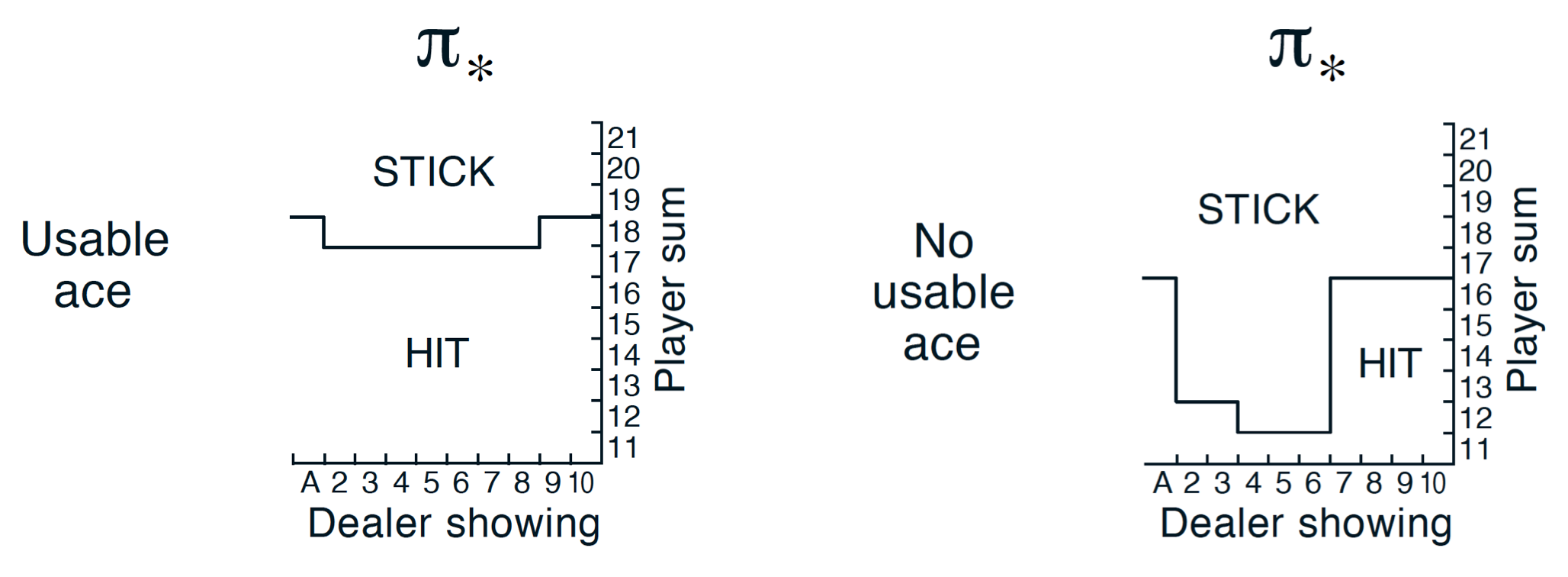
To estimate $\pi \approx \pi^\star$, we will use the on-policy first-visit Monte Carlo control method with $\epsilon-$soft policies.
ranges = [range(space.n) for space in env.observation_space.spaces]
observations = list(itertools.product(*ranges))
observation_to_index = {v: k for k, v in enumerate(observations)}
index_to_observation = {k: v for k, v in enumerate(observations)}

num_observations = len(observations)
num_actions = env.action_space.n

print(f"Number of observations: {num_observations}, number of actions: {num_actions}")
Number of observations: 704, number of actions: 2
Q = np.zeros((num_observations, num_actions))
S = np.zeros((num_observations, num_actions))
N = np.zeros((num_observations, num_actions), dtype=np.int)

policy_vector = np.random.choice(num_actions, size=num_observations)

num_episodes = 10_000_000
epsilon = 1.0
epsilon_decay = 0.999
epsilon_min = 0.25
gamma = 1.0

epsilons = []
history = []

for episode in trange(num_episodes):
    observation = env.reset()
    max_diff = 0.0
    is_terminal = False
    sequence = []
    while not is_terminal:
        index = observation_to_index[observation]
        if observation[0] <= 10:
            action = 1
        else:
            probs = np.copy(Q[index])
            best_action = policy_vector[index]
            probs = np.ones(num_actions) * epsilon / num_actions
            probs[best_action] = 1 - epsilon + (epsilon / num_actions)
            action = np.random.choice(num_actions, p=probs)
        new_observation, reward, is_terminal, _ = env.step(action)
        sequence.append((index, action, reward))
        observation = new_observation
    G = 0
    for index, action, reward in reversed(sequence):
        G = reward + gamma * G
        N[index, action] += 1
        S[index, action] += G
        old_value = Q[index, action]
        Q[index, action] = S[index, action] / N[index, action]
        policy_vector[index] = np.argmax(Q[index] + np.random.uniform(high=1e-8, size=(2,)))
        max_diff = max(max_diff, abs(Q[index, action] - old_value))
    history.append(max_diff)
    epsilons.append(epsilon)
    if episode % 1_000 == 0:
        epsilon = max(epsilon * epsilon_decay, epsilon_min)
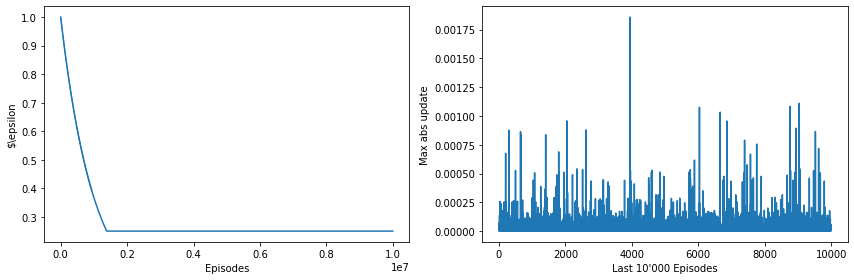
We plot the exploration rate $\epsilon$ over all the episodes and the maximum error for the last 10’000 episodes.
fig, (ax0, ax1) = plt.subplots(ncols=2, figsize=(12, 4))
ax0.plot(epsilons)
ax0.set_xlabel('Episodes')
ax0.set_ylabel('$\epsilon')
ax1.plot(history[-10_000:])
ax1.set_xlabel('Last 10\'000 Episodes')
ax1.set_ylabel('Max abs update')
fig.tight_layout()
from matplotlib import cm
from mpl_toolkits.axes_grid1 import make_axes_locatable

rows, cols = 11, 10
fig, (ax0, ax1) = plt.subplots(ncols=2)
for (ax, has_ace) in [(ax0, True), (ax1, False)]:
    image = []
    for my_sum in range(21, 10, -1):
        row = []
        for dealer in range(1, env.observation_space.spaces[1].n):
            row.append(policy_vector[observation_to_index[(my_sum, dealer, has_ace)]])
        image.append(row)

    surf = ax.matshow(image, cmap=plt.get_cmap('Pastel1', 2),
                      extent=[-1, 9, 10, -1])
    row_labels = np.arange(11, 22)
    col_labels = ['A', '2', '3', '4', '5', '6', '7', '8', '9', '10']
    surf = ax.matshow(image, cmap=plt.get_cmap('Pastel1', 2),
                      extent=[-1, 9, 10, -1])
    ax.set_xlabel('Dealer showing')
    ax.set_ylabel('Player sum')
    ax.set_xticks(np.arange(cols) - 0.5)
    ax.set_xticklabels(col_labels)
    ax.set_yticks(np.arange(rows)[::-1] - 0.5)
    ax.set_yticklabels(row_labels)
    ax.set_title(("Usable ace" if has_ace else "No usable ace"), fontsize=16)

ax0.text(0, 1, 'STICK', fontsize=12)
ax0.text(6, 8, 'HIT', fontsize=12)
ax1.text(0, 1, 'STICK', fontsize=12)
ax1.text(6, 8, 'HIT', fontsize=12)
fig.tight_layout()
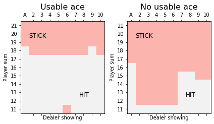
The image above is similar, yet not identical, to the one in the book from Sutton and Barto. They use a different method, which is difficult to apply to the OpenAI Gym environment, and also limit themselved to 500’000 episodes instead of the 10’000’000 used here. What we have presented here is very easy to implement and quite intuitive, but is converges slowly and is very sensitive to exploration rate and its decay.