What we will do in this article is to show how to define a non-trivial martingale that is bounded. We start by following the approach presented in Bounded Brownian Motion by P. Carr, in which a stochastic process $S(t)$ that is contained in $[0, H]$ is constructed by setting $S(t) = \varphi(X(t))$ and $X(t)$ is defined by the SDE
\[\begin{aligned} dX(t) & = \frac{\pi \sigma^2}{H^2}X(t) dt + \sigma dW(t) \\ X(0) & = X_0, \end{aligned}\]with $W(t)$ a standard Wiener process and $\varphi(x): \mathbb{R} \rightarrow \mathbb{R}$ a $C^2$ function that transforms the unbounded process $X(t)$ into $S(t) \in [0, H]$ for some $H > 0$. To define the transformation $\varphi(x)$ that makes $S(t)$ a martingale, we apply Ito’s lemma and impose a zero drift,
\[\begin{aligned} dS(t) & = d(\varphi(X(t))) \\ & = \left( \frac{\pi \sigma^2}{H^2} X(t) \varphi'(X(t)) + \frac{\sigma^2}{2}\varphi''(X(t)) \right) dt + \sigma \varphi'(X(t)) dW(t), \end{aligned}\]that is $\varphi(x)$ must satify the second-order ODE
\[\frac{\pi \sigma^2}{H^2} x \varphi'(x) + \frac{\sigma^2}{2}\varphi''(x) = 0\]with boundary conditions $\varphi(-\infty) = 0$ and $\varphi(\infty) = 1$. Setting $\psi = \varphi’$ we easily get
\[\begin{aligned} \frac{\pi \sigma^2}{H^2} x \psi(x) & = - \frac{\sigma^2}{2}\frac{d\psi(x)}{dx} \\ % \frac{d\psi(x)}{\psi} & = - \frac{2 \pi}{H^2} x dx \\ % \log(\psi(x)) & = C_1 - \frac{\pi}{H^2}x^2 \\ % \varphi'(x) & = e^{C_1} e^{-\frac{\pi}{H^2}x^2} \\ % \varphi(x) & = C_2 + e^{C_1} \int_{-\infty}^x e^{-\frac{\pi}{H^2} \zeta^2} d\zeta \\ % & = C_2 + e^{C_1} \int_{-\infty}^x e^{-\frac{1}{2} \left( \frac{\sqrt{2 \pi}}{H} \zeta \right)^2} d\zeta \\ % & = C_2 + e^{C_1} \frac{H}{\sqrt{2 \pi}}\int_{-\infty}^{\frac{\sqrt{2 \pi}}{H}x} e^{-\frac{1}{2} \eta^2} d\eta \\ % & = C_2 + e^{C_1} H \Phi\left( \frac{\sqrt{2\pi}}{H} x \right), \end{aligned}\]where $\Phi$ is the standard normal cumulative density function. From the boundary conditions we get $C_1=C_2=0$, therefore
\[\varphi(x) = H\Phi\left( \frac{\sqrt{2\pi}}{H} x \right)\]and
\[S(x) = H\Phi\left( \frac{\sqrt{2\pi}}{H} X(t) \right).\]Since $\Phi(x)$ maps $\mathbb{R}$ into $[0, 1]$, $S(t)$ is contained in $[0, H]$; for a generic $S(t) \in [L, U]$ we can easily modify the above procedure to obtain $S(t) = L + (U - L) \Phi(\sqrt{2\pi}/(U - L)X(t))$.
To generate $S(t)$ we can simulate $X(t)$ and apply $\varphi$, but we can also use the definition of $dX(t)$ we obtained through the application of Ito’s lemma. The drift is zero by construction, so we are left with
\[dS(t) = \sigma \sqrt{2\pi} \, \Phi' \left( \frac{\sqrt{2\pi}}{H} X(t) \right) dW(t).\]From the definition of $S(t)$ we have
\[\frac{\sqrt{2\pi}}{H} X(t) = \Phi^{-1} \left( \frac{S(t)}{H}\right),\]where $\Phi^{-1}$ is the inverse cumulative density function of the standard normal distribution and
\[\begin{aligned} dS(t) & = \sigma \sqrt{2\pi} \Phi'\left( \Phi^{-1}\left( \frac{S(t}{H} \right) \right) \\ % & = \sigma \exp\left( -\frac{1}{2} \left( \Phi^{-1} \left(\frac{S(t)}{H}\right)\right)^2 \right). \end{aligned}\]From the above equation we see that $S(t)$ is a time-homogeneous driftless diffusion process, with a diffusion coefficient that is largest when $(\Phi^{-1})^2$ is minimal, that is for $S(t) = \frac{1}{2} H$ – that is, the point in between the bounds 0 and $H$ – and goes to zero quickly near 0 and near $H$, meaning that the process becomes more deterministic as $S(t) \rightarrow 0$ and $S(t) \rightarrow H$.
Let’s simulate this process and numerically check the martingale property.
import matplotlib.pylab as plt
import numpy as np
from scipy.stats import norm
plt.style.use('ggplot')
S_0, H, σ, T = 0.6, 1.0, 1.0, 10.0
num_steps = 501
t_all = np.linspace(0, H, num_steps + 1)
Φ, π = norm.cdf, np.pi
def transform(x):
    return H * Φ(np.sqrt(2 * π) / H * x)
def generate_path():
    X = H / np.sqrt(2 * π) * norm.ppf(S_0 / H)
    path = [S_0]
    for Δt in np.diff(t_all):
        Z = norm.rvs()
        X = X + π * σ**2 / H**2 * X * Δt + σ * np.sqrt(Δt) * Z
        path.append(transform(X))
    return path
plt.figure(figsize=(12, 4))
for _ in range(50):
    plt.plot(t_all, generate_path())
plt.xlabel('t')
plt.ylabel('S(t)');
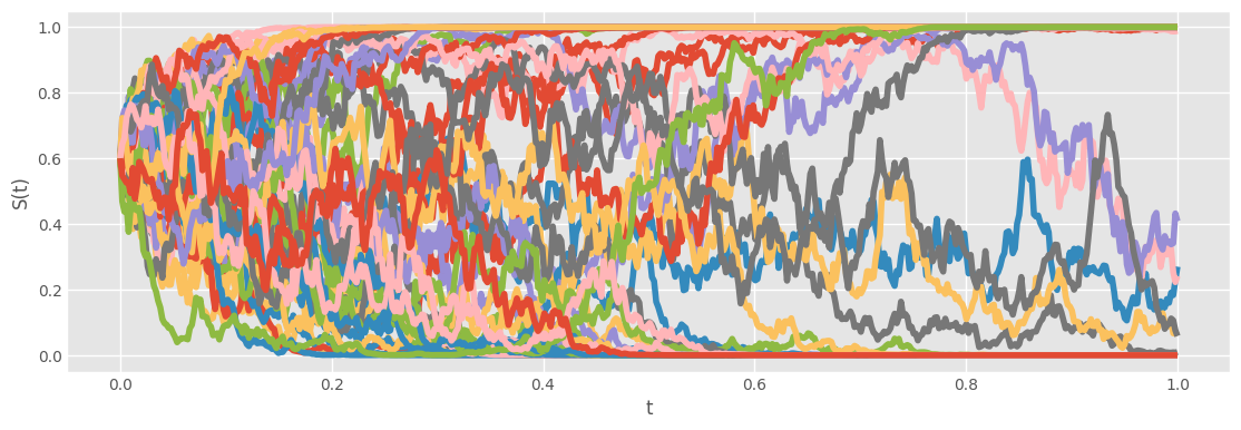
It is easy to see from the above plot that there are two states, one at 0 and the other at $H=1$. The process remains a martingale, but after some time the paths are very close to the bounds.
Another choice for the drift coefficient for which we have analytically tractable expression was discussed in Option Pricing: Channels, Target Zones and Sideways Markets by Z. Kakushadze and reads
\[\mu(x) = \nu \sigma^2 \tanh(\nu(x - x^\star)),\]for which we get
\[\begin{aligned} \varphi'(x) & = C \exp\left( -\frac{2}{\sigma^2} \int_{-\infty}^x \mu(\zeta) d\zeta \right) \\ % & = C \exp \left( -2 \nu \int_{-\infty}^x \tanh(\nu(\zeta - x^\star)) d\zeta \right) \\ % & = C \exp\left( -2 \int_{-\infty}^{\nu(x - x^\star)} \tanh(\eta)d\eta \right) \\ % & = C \exp\left( -2 \ln \cosh(\nu(x - x^\star)) \right) \\ % & = C \exp\left( \ln(\cosh(\nu(x - x^\star))^{-2} \right) \\ % & = \frac{C}{\cosh^2(\nu(x - x^\star))} \end{aligned}\]and therefore
\[\varphi(x) = A + B \tanh(\nu(x - x^\star)),\]where $A$ and $B$ are two constants defined such that the unattainable boundaries are $A - B$ and $A+B$, while $x^\star$ is the value of the mean. We also note that this process is mean-repelling.
The probability density $p(x, t)$ for a process starting at $x_0$ at $t=0$ can be computed from the Fokker-Planck equation
\[\frac{\partial}{\partial t}[(x, t)] + \frac{\partial}{\partial x}\left( \mu(x)p(x, t) \right) - \frac{\sigma^2}{2} \frac{\partial^2}{\partial x^2}p(x, t) = 0\]and reads
\[p(x, t) = \frac{1}{\sqrt{2\pi} \sigma} \frac{\cosh(\nu(x - x^\star))}{\cosh(\nu(x_0 - x^\star)} \exp\left( -\frac{(x - x_0)^2}{2 \sigma^2 t} - \frac{\sigma^2 \nu^2 t}{2} \right)\]meaning that $p$ is a linear combination of two Gaussians.