Following our previous post on PINNs on a one-dimensional Laplacian, we take a step further and solve something a bit more challenging and interesting: the Burgers’ equation,
\[\frac{\partial u(t, x)}{\partial t} + u(t, x) \frac{\partial u(t, x)}{\partial x} = \nu \frac{\partial^2 u(t, x)}{\partial x^2},\]which is well understood and documented in the literature. The meaning of the symbols is:
- $x$ is the spatial coordinate;
- $t$ is the temporal coordinate;
- $u(x,t)$ is the speed of fluid at the indicated spatial and temporal coordinates $(x, t)$; and
- $\nu$ viscosity of fluid.
When $\nu = 0$ we have the inviscid Burgers’ equation; we consider $\nu$ to be small but positive, obtaining the viscous flavor. This equation can be seen as a simplified framework to study fluid dynamics, where indeed $\nu$ tends to be small and the nonlinear term $u(t, x) \frac{\partial u(t, x)}{\partial x}$ introduces non-negligible complexities into the equations. This PDE is of parabolic type (when $\nu > 0$, which is the case we consider) and it is well known that regions with very steep gradients can develop even from benign initial and boundary conditions.
Following this website, we assume $x \in (-1, 1)$ and $t \in (0, 1)$, initial conditions
\[u(0, x) = - \sin(\pi x)\]and the boundary conditions
\[u(t, -1) = u(t, 1) = 0.\]Finally, the parameter $\nu$ is set to a small number,
\[\nu = \frac{0.01}{\pi}.\]Compared to the solution of the Laplacian, here we have two input variables, $t$ and $x$. We also need to take into account the initial and the boundary conditions.
import matplotlib.pylab as plt
import numpy as np
import torch
from torch import nn
from torch.autograd import grad
The network is quite simple, composed by linear layers with tanh activation function.
class Model(nn.Module):
    def __init__(self):
        super(Model, self).__init__()
        self.layer1  = nn.Linear(2, 80)
        self.layer2  = nn.Linear(80, 80)
        self.layer3  = nn.Linear(80, 40)
        self.layer4  = nn.Linear(40, 1)
        self.activation  = nn.Tanh()
        for m in self.modules():
            if isinstance(m, nn.Linear):
                nn.init.normal_(m.weight, mean=0, std=0.1)

    def forward(self, x, t):
        u = torch.cat((x, t), 1)
        u = self.activation(self.layer1(u))
        u = self.activation(self.layer2(u))
        u = self.activation(self.layer3(u))
        u = self.layer4(u)
        return u
def flat(x):
    m = x.shape[0]
    return [x[i] for i in range(m)]
π = np.pi
μ = torch.tensor(0.01 / π)
A few helper functions are used to define the internal equations, the initial conditions, and the boundary conditions.
def equations(model, x, t):
    u = model(x, t)
    u_t = grad(flat(u), t, create_graph=True, allow_unused=True)[0]
    u_x = grad(flat(u), x, create_graph=True, allow_unused=True)[0]
    u_xx = grad(flat(u_x), x, create_graph=True, allow_unused=True)[0]
    return u_t, -u * u_x + μ * u_xx
def initial_conditions(model, x, t):
    u = model(x, t)
    return u, -torch.sin(π * x)
def boundary_conditions(model, x, t):
    u = model(x, t)
    return u, torch.zeros_like(u)
We also need to sample randomly from the (internal) domain $\Omega$, as well as from the appropriate domains for the initial and boundary conditions. A few helper functions are created for this aim.
def get_t(num_points, requires_grad):
    # t points are in the (0, 1) interval
    return torch.rand((num_points, 1), requires_grad=requires_grad, dtype=torch.float32)
def get_x(num_points, requires_grad):
    # x points are in the (-1, 1) interval
    return torch.rand((num_points, 1), requires_grad=requires_grad, dtype=torch.float32) * 2 - 1
def internal_points(num_points):
    return get_x(num_points, True), get_t(num_points, True)
def initial_points(num_points):
    x = get_x(num_points, False)
    return x, torch.zeros_like(x)
def boundary_points(num_points):
    t = get_t(num_points, False)
    x = torch.ones_like(t)
    x[:num_points // 2, :] *= -1
    return x, t
num_epochs = 10_000
num_points = 256
num_initial_points = 32
num_boundary_points = 32
λ = 10.0

model = Model()
optimizer = torch.optim.Adam(model.parameters(), lr=0.0005)
history = []
loss_fn = nn.MSELoss()

for epoch in range(num_epochs):
    optimizer.zero_grad()
    x_internal, t_internal = internal_points(num_points)
    lhs_internal, rhs_internal = equations(model, x_internal, t_internal)

    x_initial, t_initial = initial_points(num_initial_points)
    lhs_initial, rhs_initial = initial_conditions(model, x_initial, t_initial)

    x_boundary, t_boundary = boundary_points(num_boundary_points)
    lhs_boundary, rhs_boundary = boundary_conditions(model, x_boundary, t_boundary)

    loss = loss_fn(lhs_internal, rhs_internal) \
        + λ * loss_fn(lhs_initial, rhs_initial) \
        + λ * loss_fn(lhs_boundary, rhs_boundary)
    loss.backward()
    optimizer.step()
    history.append(loss.detach().numpy())
    if (epoch + 1) % 1_000 == 0:
        print(epoch + 1, history[-1])
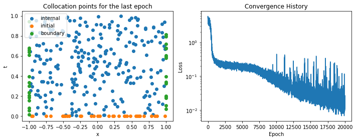
The figure below shows, on the left, the collocation points on the domain for the last epoch (they are selected randomly at each epoch), and on the right the convergence history of the loss function.
to_numpy = lambda x: x.detach().flatten().numpy()
fig, (ax0, ax1) = plt.subplots(figsize=(10, 4), ncols=2)
ax0.scatter(to_numpy(x_internal), to_numpy(t_internal), label='internal')
ax0.scatter(to_numpy(x_initial), to_numpy(t_initial), label='initial')
ax0.scatter(to_numpy(x_boundary), to_numpy(t_boundary), label='boundary')
ax0.legend(loc='upper left')
ax0.set_xlabel('x')
ax0.set_ylabel('t')
ax0.set_title('Collocation points for the last epoch')
ax1.semilogy(history)
ax1.set_xlabel('Epoch')
ax1.set_ylabel('Loss')
ax1.set_title('Convergence History')
fig.tight_layout()
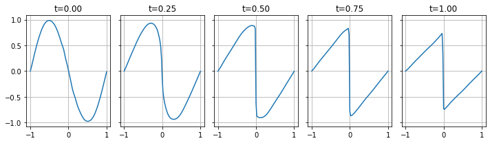
fig, axes = plt.subplots(figsize=(10, 3), ncols=5, nrows=1, sharey=True)
for t, ax in zip([0.0, 0.25, 0.5, 0.75, 1.0], axes):
    x = torch.linspace(-1, 1, 101).reshape(-1, 1)
    z = model(x, torch.ones_like(x) * t)
    ax.plot(x.numpy(), z.detach().numpy())
    ax.set_title(f't={t:.2f}')
    ax.grid()
fig.tight_layout()