In this article we look at the constant elasticity of variance (CEV) model of Cox (1975), which allows the instantaneous variance of the asset returns to depend ont he asset price level, thus exhibiting an implied volatility skew.
Under the risk-neutral measure $\mathbb{Q}$, the model reads
\[dS(t) = (r - q)S(t) dt + \delta S(t)^{\beta/2} dW(t),\]where $r$ is the instantaneous riskless interest rate, which is assumed to be constant, and $q$ is the dividend yield for the underling asset price, assumed to be constant as well. The local volatility function is then given by
\[\sigma(s) = \delta s^{\beta - 1},\]where $\beta$ is a real number and $\delta > 0$. THe name of the model is understood if we consider
\[\frac{dv(S(t))}{S(t)} = (\beta - 2) \frac{dS(t)}{S(t)},\]where $v(s) = \delta^2 s^{\beta/2 - 1}$ is the instantenous variance. The model parameter $\delta$ can be interpreted as the parameter fixing the initial level of the volatility at $t=0$,
\[\sigma(S_0) = \delta S_0^{\beta/2 - 1},\]where $S_0$ is given, that is
\[\delta = \frac{\sigma(S_0)}{S_0^{\beta - 1}}.\]For $\beta = 2$ we recover the Black-Scholes model; for $\beta > 2$ the volatility is an increasing function of the asset price, while for $\beta < 2$ it is a decreasing function. For $\beta=1$ we recover the square-root diffusion model of Cox and Ross (76).
The call price is expressed in terms of the non-central $\chi^2$ distribution as
\[C = \begin{cases} S(t) e^{-q T} Q(2y; 2 + \frac{2}{2 - \beta}, 2x) - K e^{-r T} \left[ 1 - Q(2x; \frac{2}{2 - \beta}, 2y) \right] % & \beta < 2 \\ % S(t) % & \beta > 2 \end{cases}\]from collections import namedtuple
import matplotlib.pylab as plt
import numpy as np
from scipy.stats import norm, ncx2
Model = namedtuple('Model', 'S_0, r, q, δ, β')
Vanilla = namedtuple('Vanilla', 'N, K, T, is_call')
def generate_paths(model, schedule, num_paths):
    S_0, r, q, 𝛿, β = model
    num_steps = len(schedule) - 1
    retval = [np.ones((num_paths, )) * S_0]
    S_t = retval[0]
    W = norm.rvs(size=(num_paths, num_steps))
    t = 0.0
    for i in range(0, num_steps):
        Δt = schedule[i + 1] - schedule[i]
        t = t + Δt
        sqrt_Δt =  np.sqrt(Δt)
        σ = 𝛿 * np.power(S_t, β / 2 - 1)
        S_t = S_t + (r - q - 0.5 * σ**2) * Δt + σ * sqrt_Δt * W[:, i]
        retval.append(S_t)
    return np.vstack(retval)
model = Model(S_0=1.0, r=0.05, q=0.03, δ=0.25, β=2.5)
vanilla = Vanilla(N=1.0, K=model.S_0, T=1.0, is_call=True)
schedule = np.linspace(0, vanilla.T, 101)
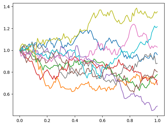
Let’s plot a few paths.
paths = generate_paths(model, schedule, 100)
for i in range(10):
    plt.plot(schedule, paths[:, i])
num_paths = 100_000
paths = generate_paths(model, schedule, num_paths)
S_T = paths[-1, :]
payoffs = np.maximum(S_T - vanilla.K, 0.0)
df = np.exp(-vanilla.T * model.r)
price, std = df * payoffs.mean(), df * payoffs.std() / np.sqrt(num_paths)
print(f'Monte Carlo price: {price:2f}')
print(f'95% confidence interval: ({price - 1.96 * std}, {price + 1.96 * std})')
Monte Carlo price: 0.088335
95% confidence interval: (0.08748103223320207, 0.08918885672076678)