The CIFAR-10 data set is composed of 60,000 32x32 colour images, 6,000 images per class, so 10 categories in total. The training set is made up of 50,000 images, while the remaining 10,000 make up the testing set.
The categories are: airplane, automobile, bird, cat, deer, dog, frog, horse, ship and truck.
More information regarding the CIFAR-10 and CIFAR-100 data sets can be found here.
import torch
import matplotlib.pyplot as plt
import numpy as np
import torch.nn.functional as F
from torch import nn
from torchvision import datasets, transforms
device = torch.device("cuda:0" if torch.cuda.is_available() else "cpu")
print(f"Using device '{device}'.")
Using device 'cuda:0'.
PyTorch provides data loaders for common data sets used in vision applications, such as MNIST, CIFAR-10 and ImageNet through the torchvision package. Other handy tools are the torch.utils.data.DataLoader that we will use to load the data set for training and testing and the torchvision.transforms, which we will use to compose a two-step process to prepare the data for use with the CNN.
transform_train = transforms.Compose([
       transforms.Resize((32,32)),
       transforms.RandomHorizontalFlip(),
       transforms.RandomRotation(10),
       transforms.RandomAffine(0, shear=10, scale=(0.8,1.2)),
       transforms.ColorJitter(brightness=0.2, contrast=0.2, saturation=0.2),
       transforms.ToTensor(),
       transforms.Normalize((0.5, 0.5, 0.5), (0.5, 0.5, 0.5))
])

transform_valid = transforms.Compose([
       transforms.Resize((32,32)),
       transforms.ToTensor(),
       transforms.Normalize((0.5, 0.5, 0.5), (0.5, 0.5, 0.5))
])

dataset_train = datasets.CIFAR10(root='./data', train=True, download=True, transform=transform_train)
dataset_valid = datasets.CIFAR10(root='./data', train=False, download=True, transform=transform_valid)
print(f"Using {len(dataset_train)} images for training and {len(dataset_valid)} for validation.")

loader_train = torch.utils.data.DataLoader(dataset_train, batch_size=100, shuffle=True)
loader_valid = torch.utils.data.DataLoader(dataset_valid, batch_size=100, shuffle=False)
Files already downloaded and verified
Files already downloaded and verified
Using 50000 images for training and 10000 for validation.
def im_convert(tensor):
    image = tensor.cpu().clone().detach().numpy()
    image = image.transpose(1, 2, 0)
    image = image * np.array((0.5, 0.5, 0.5)) + np.array((0.5, 0.5, 0.5))
    image = image.clip(0, 1)
    return image
classes = ('plane', 'car', 'bird', 'cat', 'deer', 'dog', 'frog', 'horse', 'ship', 'truck')
dataiter = iter(loader_train)
images, labels = dataiter.next()
fig = plt.figure(figsize=(25, 4))

for idx in np.arange(20):
    ax = fig.add_subplot(2, 10, idx+1, xticks=[], yticks=[])
    plt.imshow(im_convert(images[idx]))
    ax.set_title(classes[labels[idx].item()])

class LeNet(nn.Module):

    def __init__(self):
        super().__init__()
        self.conv1 = nn.Conv2d(3, 16, 3, 1, padding=1)
        self.conv2 = nn.Conv2d(16, 32, 3, 1, padding=1)
        self.conv3 = nn.Conv2d(32, 64, 3, 1, padding=1)
        self.fc1 = nn.Linear(4*4*64, 500)
        self.dropout1 = nn.Dropout(0.5)
        self.fc2 = nn.Linear(500, 10)

    def forward(self, x):
        x = F.relu(self.conv1(x))
        x = F.max_pool2d(x, 2, 2)
        x = F.relu(self.conv2(x))
        x = F.max_pool2d(x, 2, 2)
        x = F.relu(self.conv3(x))
        x = F.max_pool2d(x, 2, 2)
        x = x.view(-1, 4*4*64)
        x = F.relu(self.fc1(x))
        x = self.dropout1(x)
        x = self.fc2(x)
        return x
model = LeNet().to(device)
model
LeNet(
  (conv1): Conv2d(3, 16, kernel_size=(3, 3), stride=(1, 1), padding=(1, 1))
  (conv2): Conv2d(16, 32, kernel_size=(3, 3), stride=(1, 1), padding=(1, 1))
  (conv3): Conv2d(32, 64, kernel_size=(3, 3), stride=(1, 1), padding=(1, 1))
  (fc1): Linear(in_features=1024, out_features=500, bias=True)
  (dropout1): Dropout(p=0.5, inplace=False)
  (fc2): Linear(in_features=500, out_features=10, bias=True)
)
criterion = nn.CrossEntropyLoss()
optimizer = torch.optim.Adam(model.parameters(), lr = 1e-3)
epochs = 30
loss_history_train, loss_history_valid = [], []
accuracy_history_train, accuracy_history_valid = [], []

for epoch in range(1, epochs + 1):

    total_loss_train, total_accuracy_train = 0.0, 0.0
    total_loss_valid, total_accuracy_valid = 0, 0

    for inputs, labels in loader_train:
        inputs = inputs.to(device)
        labels = labels.to(device)
        outputs = model(inputs)
        loss = criterion(outputs, labels)

        optimizer.zero_grad()
        loss.backward()
        optimizer.step()

        _, preds = torch.max(outputs, 1)
        total_loss_train += loss.item()
        total_accuracy_train += torch.sum(preds == labels.data).item()
    else:
        with torch.no_grad():
            for inputs, labels in loader_valid:
                inputs = inputs.to(device)
                labels = labels.to(device)
                outputs = model(inputs)
                loss = criterion(outputs, labels)

                _, preds = torch.max(outputs, 1)
                total_loss_valid += loss.item()
                total_accuracy_valid += torch.sum(preds == labels.data).item()

        total_loss_train /= len(dataset_train)
        total_accuracy_train /= len(dataset_train)
        loss_history_train.append(total_loss_train)
        accuracy_history_train.append(total_accuracy_train)

        total_loss_valid /= len(dataset_valid)
        total_accuracy_valid /= len(dataset_valid)
        loss_history_valid.append(total_loss_valid)
        accuracy_history_valid.append(total_accuracy_valid)

        print(f"epoch {epoch:2d}, train: loss = {total_loss_train:.4f}, accuracy = {total_accuracy_train:.4%}")
        print(f"          valid: loss = {total_loss_valid:.4f}, accuracy = {total_accuracy_valid:.4%}")
        print()
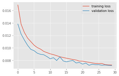
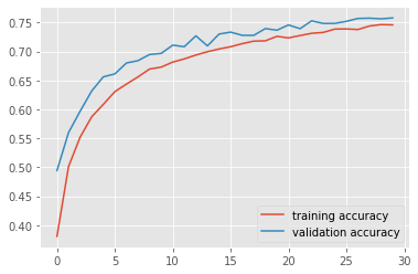
epoch  1, train: loss = 0.0169, accuracy = 38.0500%
          valid: loss = 0.0138, accuracy = 49.4200%

epoch  2, train: loss = 0.0138, accuracy = 50.1160%
          valid: loss = 0.0122, accuracy = 55.9900%

epoch  3, train: loss = 0.0125, accuracy = 55.1940%
          valid: loss = 0.0113, accuracy = 59.6800%

epoch  4, train: loss = 0.0116, accuracy = 58.7160%
          valid: loss = 0.0104, accuracy = 63.1800%

epoch  5, train: loss = 0.0110, accuracy = 60.8500%
          valid: loss = 0.0098, accuracy = 65.6200%

epoch  6, train: loss = 0.0104, accuracy = 63.0660%
          valid: loss = 0.0096, accuracy = 66.1300%

epoch  7, train: loss = 0.0101, accuracy = 64.3620%
          valid: loss = 0.0092, accuracy = 68.0100%

epoch  8, train: loss = 0.0098, accuracy = 65.6120%
          valid: loss = 0.0090, accuracy = 68.4200%

epoch  9, train: loss = 0.0094, accuracy = 66.9700%
          valid: loss = 0.0089, accuracy = 69.4800%

epoch 10, train: loss = 0.0092, accuracy = 67.2980%
          valid: loss = 0.0086, accuracy = 69.6700%

epoch 11, train: loss = 0.0090, accuracy = 68.1720%
          valid: loss = 0.0083, accuracy = 71.1000%

epoch 12, train: loss = 0.0089, accuracy = 68.7220%
          valid: loss = 0.0084, accuracy = 70.8300%

epoch 13, train: loss = 0.0088, accuracy = 69.3860%
          valid: loss = 0.0080, accuracy = 72.7100%

epoch 14, train: loss = 0.0086, accuracy = 69.9660%
          valid: loss = 0.0086, accuracy = 70.9700%

epoch 15, train: loss = 0.0085, accuracy = 70.4320%
          valid: loss = 0.0079, accuracy = 73.0100%

epoch 16, train: loss = 0.0083, accuracy = 70.8220%
          valid: loss = 0.0078, accuracy = 73.3500%

epoch 17, train: loss = 0.0082, accuracy = 71.3540%
          valid: loss = 0.0079, accuracy = 72.8000%

epoch 18, train: loss = 0.0081, accuracy = 71.7980%
          valid: loss = 0.0080, accuracy = 72.7900%

epoch 19, train: loss = 0.0081, accuracy = 71.8480%
          valid: loss = 0.0076, accuracy = 73.9600%

epoch 20, train: loss = 0.0079, accuracy = 72.6180%
          valid: loss = 0.0077, accuracy = 73.6800%

epoch 21, train: loss = 0.0079, accuracy = 72.3480%
          valid: loss = 0.0074, accuracy = 74.5900%

epoch 22, train: loss = 0.0078, accuracy = 72.7600%
          valid: loss = 0.0076, accuracy = 73.9400%

epoch 23, train: loss = 0.0077, accuracy = 73.1480%
          valid: loss = 0.0072, accuracy = 75.3000%

epoch 24, train: loss = 0.0076, accuracy = 73.2980%
          valid: loss = 0.0074, accuracy = 74.8500%

epoch 25, train: loss = 0.0075, accuracy = 73.8720%
          valid: loss = 0.0073, accuracy = 74.8600%

epoch 26, train: loss = 0.0075, accuracy = 73.9000%
          valid: loss = 0.0073, accuracy = 75.2100%

epoch 27, train: loss = 0.0075, accuracy = 73.8000%
          valid: loss = 0.0072, accuracy = 75.7100%

epoch 28, train: loss = 0.0073, accuracy = 74.4040%
          valid: loss = 0.0073, accuracy = 75.7600%

epoch 29, train: loss = 0.0073, accuracy = 74.6500%
          valid: loss = 0.0072, accuracy = 75.6500%

epoch 30, train: loss = 0.0073, accuracy = 74.6040%
          valid: loss = 0.0072, accuracy = 75.8000%
plt.style.use('ggplot')
plt.plot(loss_history_train, label='training loss')
plt.plot(loss_history_valid, label='validation loss')
plt.legend();

plt.plot(accuracy_history_train, label='training accuracy')
plt.plot(accuracy_history_valid, label='validation accuracy')
plt.legend();

# prepare to count predictions for each class
correct_pred = {classname: 0 for classname in classes}
total_pred = {classname: 0 for classname in classes}
confusion_matrix = np.zeros([10, 10], int)

# again no gradients needed
with torch.no_grad():
    for images, labels in loader_valid:
        images = images.to(device)
        labels = labels.to(device)
        outputs = model(images)
        _, predictions = torch.max(outputs, 1)
        # collect the correct predictions for each class
        for label, prediction in zip(labels, predictions):
            if label == prediction:
                correct_pred[classes[label]] += 1
            total_pred[classes[label]] += 1
        for i, l in enumerate(labels):
            confusion_matrix[l.item(), predictions[i].item()] += 1

# print accuracy for each class
for classname, correct_count in correct_pred.items():
    accuracy = 100 * float(correct_count) / total_pred[classname]
    print(f'Accuracy for class: {classname:5s} is {accuracy:.1f} %')
Accuracy for class: plane is 77.7 %
Accuracy for class: car   is 89.5 %
Accuracy for class: bird  is 65.5 %
Accuracy for class: cat   is 62.1 %
Accuracy for class: deer  is 65.9 %
Accuracy for class: dog   is 71.8 %
Accuracy for class: frog  is 76.5 %
Accuracy for class: horse is 83.2 %
Accuracy for class: ship  is 84.0 %
Accuracy for class: truck is 80.6 %
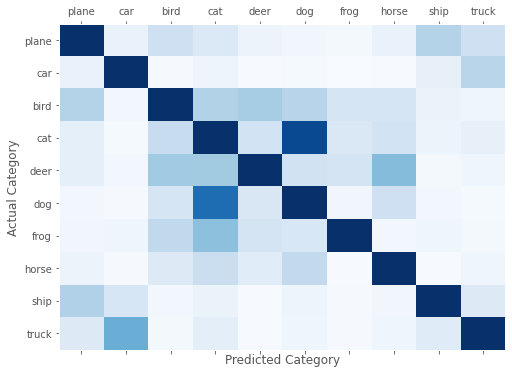
The model performed much better than random guessing, which would give us an accuracy of 10% since there are ten categories in CIFAR-10. Let us now use the confusion matrix to compute the accuracy of the model per category.
Let us visualise the confusion matrix to determine common misclassifications.
fig, ax = plt.subplots(1,1,figsize=(8,6))
ax.matshow(confusion_matrix, aspect='auto', vmin=0, vmax=200, cmap=plt.get_cmap('Blues'))
plt.ylabel('Actual Category')
plt.yticks(range(10), classes)
plt.xlabel('Predicted Category')
plt.xticks(range(10), classes)
plt.grid();

dataiter = iter(loader_valid)
images, labels = dataiter.next()
images = images.to(device)
labels = labels.to(device)
output = model(images)
_, preds = torch.max(output, 1)

fig = plt.figure(figsize=(25, 4))

for idx in np.arange(20):
  ax = fig.add_subplot(2, 10, idx+1, xticks=[], yticks=[])
  plt.imshow(im_convert(images[idx]))
  ax.set_title("{} ({})".format(str(classes[preds[idx].item()]), str(classes[labels[idx].item()])), color=("green" if preds[idx]==labels[idx] else "red"))

import PIL.ImageOps
import requests
from PIL import Image

url = 'https://th.bing.com/th/id/OIP.-UOKKiatX4pK4AfW4JIMpQHaF2?w=228&h=180&c=7&r=0&o=5&pid=1.7'
response = requests.get(url, stream = True)
img = Image.open(response.raw)

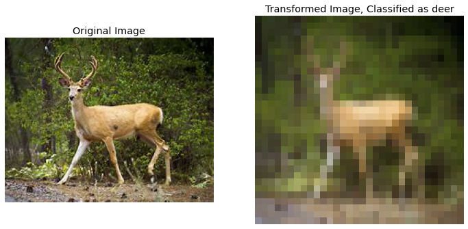
fig, (ax0, ax1) = plt.subplots(figsize=(12, 6), ncols=2)
ax0.imshow(img)
ax0.set_title('Original Image')
ax0.axis('off')

img = transform_valid(img)
ax1.imshow(im_convert(img))
image = img.to(device).unsqueeze(0)
output = model(image)
_, pred = torch.max(output, 1)
ax1.set_title(f"Transformed Image, Classified as {classes[pred.item()]}")
ax1.axis('off');
