The Cross-Entropy Method (CEM) is a derivative-free optimization techniques, originally introduced by Reuven Y. Rubinstein in 1999 article presenting an adaptive importance sampling procedure for the stimation of rate event probabilities. It can be seen as an Evolution Strategy which minimizes a cost function $\varphi(x)$ by finding a suitable “individual” $x^\star$. The individuals are sampled from a given distribution and sorted based on the cost function. A small number of “elite” candidates is selected and used to determine the parameters for the population for the next iteration. The optimization procedure involves two iterative phases:
- the generation of a set of random samples according to a specified parametrized model; and
- the updating of the model parameters, based on the best samples generated in the previous step, with cross-entropy minimization.
The method can be applied to discrete, continuous or mixed optimization, and it can be shown to be a global optimization method, particularly useful when the optimization function has many local minima. As we will see, the code is relatively compact and easy to change, and the method is based on rigorous mathematical and statistical principles.
The method was originally proposed to estimate rate-event probabilities, and in particular the value
\[\ell = \mathbb{P}[ \varphi(X) \ge \gamma ],\]where $\varphi$ can be thought of as an objective function of $X$, and the events $X$ follow a distribution defined by $f(x)$. We want to find events $X$ where our objective function $\varphi(X)$ is above some thershold $\gamma$. This can be expressed in expectations as
\[\ell = \mathbb{E}_f[\mathbb{1}_{\varphi(X) \ge \gamma}],\]where $\mathbb{1}$ is the indicator function. If this probability is very small, say smaller than $10^{−5}$, a case when $\varphi(X) \ge \gamma$ is called a rare event.
A straightforward way to estimate $\ell$ is through Monte Carlo (sometimes called in the CEM literature crude Monte Carlo), that is we draw a random sample $X_1, X_2, \ldots, X_N$ from the distribution of $X$ and use
\[\hat\ell = \frac{1}{N}\sum \mathbb{1}_{\varphi(X_i) \ge \gamma}\]as the unbiased estimate of $\ell$. However, for rare events $N$ needs to be very large in order to estimate $\ell$ accurately with a small confidence interval.
A better way is to use importance sampling. This is a well-known variance reduction technique in which the system is simulated using a different probability distribution, so as to make the rare event more likely. That is, we evaluate $\ell$ using
\[\hat\ell = \frac{1}{N} \sum_{i=1}^N \mathbb{1}_{\varphi(X_i) \ge \gamma} \frac{f(X_i)}{g_\vartheta(X_i)},\]where $g_\vartheta$ is the function that minimizes the variance of $\hat\ell$. It is well known that the best way to estimate $\ell$ is to use the change of measure with density
\[g^\star(x) := \frac{ \mathbb{1}_{\varphi(X_i) \ge \gamma} f(X) }{ \ell },\]which would produce a zero variance and will therefore yield the exact result with just one sample. Unfortunately, in order to define $g^\star$ we need to know $\ell$, which is exactly what we are looking for, so the above formula cannot be directly applied. What we can do instead is to use a function $g_\vartheta(x)$ and look for the parameters $\vartheta$ such that the distance between $g_\vartheta$ and $g^\star$ is minimized.
Given two probability distributions $g^\star$ and $g_\vartheta$ with the same support, a common notion of divergence (or distance, but not strictly in the mathematical sense) is the Kullback-Leibler divergence,
\[\begin{aligned} D_{KL}(g^\star, g_\vartheta) & = \mathbb{E}_{g^\star}\left[\log \frac{g^\star(x)}{g_\vartheta(x)} \right] \\ & = \int g^\star(x) \log g^\star(x) dx - \int g^\star(x) \log g_\vartheta(x) dx. \end{aligned}\]Since the first term does not contain $\vartheta$, the minimization of the KL divergence is equivalent to the minimization of the second term,
\[- \int g^\star(x) \log g_\vartheta(x) dx,\]which is called the cross-entropy. Because of the minus sign, this is equivalent to solving the maximization problem
\[\max_{\vartheta} \int g^\star(x) \log g_\vartheta(x) dx.\]Substituting the optimal definition of $g^\star$ and ignoring $\ell$, which does not depend on $\vartheta$, we obtain
\[\max_{\vartheta} \int \mathbb{1}_{\varphi(X_i) \ge \gamma} f(X) \log g_\vartheta(x) dx.\]which is equivalent to
\[\max_{\vartheta} \mathbb{E}_f[\mathbb{1}_{\varphi(X) \ge \gamma} \log g_\vartheta(X)].\]For some families of distributions, the above problem can be solved analytically: for normal distributions, for example, it turns out that it is equivalent to maximum likelihood estimation of the parameters. If no analytic solution is available, one can use a gradient-based method together with automatic differentiation to find a numerical solution.
The method just presented is for estimation of $\ell$, but it can be used for optimization too. Suppose the problem is to maximize some function $\varphi(x)$. We consider the associated stochastic problem of estimating
\[\mathbb{P}_f[\varphi (X) \ge \gamma]\]for a given $\gamma$ and a parametric family $g_\vartheta$. Hence, for a given $\gamma$, the goal is to find $\vartheta$ such that
\[D_{KL}(\mathbb{1}_{\varphi(X) \ge \gamma} || g_\vartheta(X))\]is minimized.
Consider a continuous optimization problem with state space $\mathcal{X} \in \mathbb{R}^n$. The sampling distribution on $\mathbb{R}^n$ can be quite arbitrary and does not need to be related to the objective function $\varphi$. Usually, a random value $X$ is generated from a Gaussian distribution, characterized by a vector of means $\mu$ and a diagonal matrix $\Sigma = \operatorname{diag}(\sigma)$ of standard deviations. At each iteration of the CE method, the vector of parameters are updated as the mean and standard deviation of the elite samples. As such, a sequence of means ${ \mu_t }$ and standard deviations ${ \sigma_t }$ are generated, such that $\lim_{t\rightarrow \infty} \mu_t = x^\star$, meaning that at the end of the algorithm we should obtain a degenerated probability density. This suggests a possible stopping criterion: the algorithm stops when all the components of $\sigma_t$ are smaller in absolute value than a certain threshold $\epsilon$.
The choice for normal distribution is motivated by the availability of fast normal random number generators and th fact that the CE miminization yields a very simple solution: each each iteration, the vector of parameters $\mu_t$ and $\sigma_t$ are updated to be the sample mean and sample standard deviation of the elite set, that is of the best performing samples.
It is often useful to perform smooth updating of the parameters, that is the parameters at the $t$-iterations are a weighted combination with the parameters of the previous iteration. For normal distributions, this reads
\[\begin{aligned} \mu_t & := \omega \mu_t + (1 − \omega) \mu_{t-1} \\ \sigma_t & := \omega \sigma_t + (1 − \omega) \sigma_{t-1}. \\ \end{aligned}\]Smoothed updating can prevent the sampling distribution from converging too quickly to a sub-optimal degenerate distribution. This is especially relevant for the multivariate Bernoulli case where, once a success probability reaches 0 or 1, it can no longer change. It is also possible to use different smoothing parameters for different components of the parameter vector (e.g., the means and the variances). Alternatively, one can inject extract variance into the sampling distribution once it has degenerated to keep exploring new areas.
The CE algorithm for continuous optimization using normal sampling is defined as follows.
First, we choose some initial values for the mean $\mu_0$ and the standard deviation $\sigma_0$ and set $t=1$.
Then, on each step, we draw $X_1, \ldots, X_N$ samples from $\mathcal{N}(\mu_{t-1}, \sigma_{t-1}^2)$ and select the indices $\mathcal{I}$ of the $N_{elite}$ best performing samples.
We update the parameters on each of the $d$ dimensions: $\forall j=1, \ldots, d$, we use
\[\begin{aligned} \mu_{t, j} & = \frac{1}{N_{elite}} \sum_{k \in \mathcal{I}} X_{k, j} \\ \sigma_{t, j}^2 & = \frac{1}{N_{elite}} \sum_{k \in \mathcal{I}} \left[ X_{k, j} - \mu_{t, j} \right]^2. \end{aligned}\]Optionally, we can perform parameter smoothing as described above.
Finally, we check for convergence: if
\[\max{|\sigma_{t, j}|} < \epsilon_{tol},\]stop and return $\mu_t$ or the overall best solution generated by the algorithm.
In the standard algorith, as detailed above, the entirety of all computed samples is discarded after each iteration. To increase efficiency, the following improvements reuse some of this information:
- one can keep the elites by adding a small fraction of the elite samples to the pool of the next iteration; and
- shift elites by storing a small fraction of the elite set and add each a random quantity.
Although potentially useful, those two tricks can also shrink the variance of the samples and provide suboptimal solutions, so only a small fraction should be kept. Another variation is to change the population size as the algorithm progresses: potentially, once we are close to an optimum, less samples will be needed, suggesting that the sample size could be related to the variance.
The implementation of the above method in Python is quite simple. We only consider multivariate normal distribution, where each sample is drawn from $n$-dimensional multivariate normal distribution with independent components. The parameter vector $\varphi$ in the CE algorithm can be taken as the $2n-$dimensional vector of means and standard deviations; in each iteration these means and standard deviations are updated according to the sample mean and sample standard deviation of the elite samples. Other choices are possible: multivariate Bernoulli distributions, or more complex models like mixture models. In doing so the updating of parameters (using maximum likelihood estimation) may no longer be trivial, but one can instead employ fast methods such as the EM algorithm to determine the parameter updates.
import matplotlib.pylab as plt
from matplotlib import cm
import numpy as np
import pandas as pd
def cem(
    func,
    µ_0: np.array,
    σ_0: np.array,
    num_samples: int,
    rarity: float,
    max_iters: int,
    omega: float,
    conv_std: float = 0.001,
    bounds = None,
):
    num_dims = len(µ_0)
    assert num_dims > 0
    assert num_dims == len(σ_0)
    assert max_iters > 0
    num_elites = int(np.floor(rarity * num_samples))
    assert num_elites > 1

    # keep track of the best solution so far
    opt_x, opt_value = None, -np.inf
    µ, σ = µ_0, σ_0

    history = []
    for iter in range(max_iters):
        samples = np.random.multivariate_normal(µ, np.diag(σ**2), num_samples)

        if bounds is not None:
            for dim in range(num_dims):
                value_min = bounds[dim][0]
                samples[samples[:, dim] < value_min] = value_min
                value_max = bounds[dim][1]
                samples[samples[:, dim] > value_max] = value_max

        values = [func(x) for x in samples]
        opt_value_new = max(values)
        if opt_value_new > opt_value:
            opt_value = opt_value_new
            opt_x = samples[values.index(opt_value)]
        gamma = sorted(values)[num_samples - num_elites]
        elites = np.array([sample for (sample, value) in zip(samples, values) if value >= gamma])
        µ_new, σ_new = elites.mean(axis=0), elites.std(axis=0)
        µ = omega * µ_new + (1.0 - omega) * µ
        σ = omega * σ_new + (1.0 - omega) * σ

        history.append({
            'iter': iter,
            'gamma': gamma,
            'opt_x': opt_x,
            'opt_value': opt_value,
            'µ': µ,
            'σ': σ,
        })

        if abs(max(σ)) < conv_std:
            break

    return opt_x, opt_value, history
The CE method is fairly robust with respect to the choice of the parameters. The rarity parameter $\rho$ is typically chosen between 0.01 and 0.1. The number of elite samples $N_e = \rho N$ should be large enough to obtain a reliable parameter update. As a rule of thumb, if the dimension of $\varphi$ is $d$, the number of elites should be in the order of $10 d$ or higher.
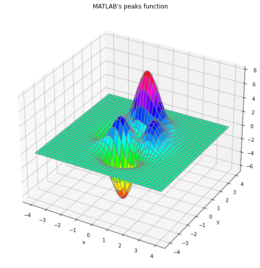
As a first test, we consider MATLAB’s peaks function, a simple two-dimensional function with two local maxima and a global one.
\[\varphi(x, y) = 3(1-x)^2 e^{-x^2 - (y+1)^2} - 10 \left(\frac{x}{5} - x^3 - y^5\right) e^{-x^2-y^2} - \frac{1}{3} e^{-(x+1)^2 - y^2}\]in $[-4, 4] \times [-4, 4]$. It has three local maxima and three local minima, with a global maximum at $(x^\star, y^\star) \sim (−0.0093, 1.58)$, with $\varphi(x^\star, y^\star) \sim 8.1$, and the other two local maximum at $\varphi(−0.46, −0.63) \sim 3.78$ and $\varphi(1.29, −0.0049) \sim 3.59$.
Depending on the starting point, gradient-based optimizer may get stuck in a local maximum, while CEM manages to easily find the global maximum.
def peaks(X):
    x, y = X
    return 3 * (1 - x)**2 * np.exp(-x**2 - (y + 1)**2) \
        - 10 * (x / 5 - x**3 - y**5) * np.exp(-x**2 - y**2) \
        - 1 / 3 * np.exp(-(x + 1)**2 - y**2)
X, Y = np.meshgrid(np.linspace(-4, 4, 201), np.linspace(-4, 4, 201))
Z = peaks([X, Y])
fig = plt.figure(figsize=(20, 20))
ax = fig.add_subplot(1,2,1, projection='3d')
ax.plot_surface(X, Y, Z, cmap=cm.hsv, linewidth=1, antialiased=True, edgecolors='grey')
ax.set_xlabel('x')
ax.set_ylabel('y')
ax.set_title("MATLAB's peaks function");
To solve the problem with CEM we must specify the vector of initial means $µ_0$ and standard deviations $σ_0$ of the 2-dimensional Gaussian sampling distribution. While $µ_0$ is largely arbitrary (unless we have a hint of the location of the maximum), $σ_0$ must be large enough such that the sampled points cover the domain of interest. Following the values given in documentation for the CEoptim R package, page 9, we take $µ_0 = (−3, −3)$ and $σ_0 = (10, 10)$.
np.random.seed(1234)
µ_0 = np.array([-3.0, -3.0])
σ_0 = np.array([10.0, 10.0])
opt_x, opt_value, history = cem(peaks, µ_0, σ_0, num_samples=100, rarity=0.1, max_iters=10, omega=1)
print(f'# iterations:', len(history))
print(f'optimal point: f({opt_x[0]:.4f}, {opt_x[1]:.4f}) = {opt_value:.4f}')
# iterations: 8
optimal point: f(-0.0093, 1.5812) = 8.1062
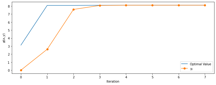
The method converges quickly, getting very close to the maximum almost immediately.
df = pd.DataFrame.from_dict(history)
fig, ax = plt.subplots(figsize=(10, 4))
ax.plot(df.opt_value, label='Optimal Value')
ax.plot(df.gamma, 'o-', label='$\gamma_t$')
ax.set_xlabel('Iteration')
ax.set_ylabel(r'$\varphi(x, y)$')
ax.legend()
fig.tight_layout();
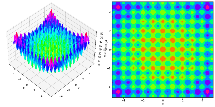
As second example, we use the two-dimensional Rastrigin’s function, for which we look for the maximum $x^\star$, located around $[\pm 4.52299366…,…,\pm 4.52299366…]$, with $f(x^\star) \sim 80.70658039$.
class Rastrigin:

    def __init__(self, n, A=10.0):
        self.n = n
        self.A = A

    def __call__(self, x):
        retval = self.A * self.n
        for i in range(self.n):
            retval += (x[i]**2 - self.A * np.cos(2 * np.pi * x[i]))
        return retval
x = np.linspace(-5.12, 5.12, 1001)
y = np.linspace(-5.12, 5.12, 1001)
xgrid, ygrid = np.meshgrid(x, y)
xy = np.stack([xgrid, ygrid])

fig = plt.figure(figsize=(12, 6))
ax = fig.add_subplot(121, projection='3d')
ax.view_init(45, -45)
ax.plot_surface(xgrid, ygrid, Rastrigin(2)(xy), cmap='hsv')
ax.set_xlabel('x')
ax.set_ylabel('y')
ax.set_zlabel('rastrigin(x, y)')

ax = fig.add_subplot(122)
ax.contourf(xgrid, ygrid, rastrigin(xy), cmap='hsv')
ax.set_xlabel('x')
ax.set_ylabel('y')

fig.tight_layout()
np.random.seed(1234)
µ_0 = np.array([0.0] * 2)
σ_0 = np.array([2.0] * 2)
bounds = [(-5.12, 5.12)] * 2
opt_x, opt_value, history = cem(Rastrigin(2), µ_0, σ_0, num_samples=100, rarity=0.1,
                                max_iters=100, omega=1, bounds=bounds)
print(f'# iterations:', len(history))
print(f'optimal value = {opt_value:.4f}')
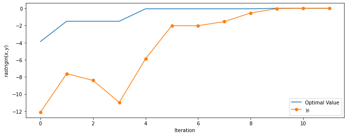
# iterations: 14, optimal value: 80.7066
The method converges is about ten iterations and provides one of the correct values (with the others begin different only for the signs).
df = pd.DataFrame.from_dict(history)
fig, ax = plt.subplots(figsize=(10, 4))
ax.plot(df.opt_value, label='Optimal Value')
ax.plot(df.gamma, 'o-', label='$\gamma_t$')
ax.set_xlabel('Iteration')
ax.set_ylabel(r'$rastrigin(x, y)$')
ax.legend()
fig.tight_layout();
In the general case of $n=3, 4, \ldots, 9$, for which the optimal values are known, we see that the algorithm works quite well up to $n=7$ and fails with the provided parameters for $n=8$ and $n=9$. We consider the test to be successful if the absolute distance between the computed solution and the exact one is less than $10^{-4}$, use a rarity parameter of 0.01, parameter smoothing, and number of samples defined as $1000 n$.
exact_opt_values = {
    1: 40.35329019,
    2: 80.70658039,
    3: 121.0598706,
    4: 161.4131608,
    5: 201.7664509,
    6: 242.1197412,
    7: 282.4730314,
    8: 322.8263216,
    9: 363.1796117,
}
for num_dims in range(3, 10):
    np.random.seed(1234)
    µ_0 = np.array([0.0] * num_dims)
    σ_0 = np.array([3.0] * num_dims)
    bounds = [(-5.12, 5.12)] * num_dims
    opt_x, opt_value, history = cem(Rastrigin(num_dims), µ_0, σ_0, num_samples=1000 * num_dims, rarity=0.01,
                                    max_iters=100, omega=0.9, bounds=bounds)
    diff = abs(opt_value - exact_opt_values[num_dims])
    status = 'OK' if diff < 1e-4 else 'failed'
    print(f'n = {num_dims}, # iterations: {len(history)}, optimal value: {opt_value:.4f}, diff: {diff:.4f} -- {status}')
n = 3, # iterations: 14, optimal value: 121.0599, diff: 0.0000 -- OK
n = 4, # iterations: 23, optimal value: 161.4132, diff: 0.0000 -- OK
n = 5, # iterations: 25, optimal value: 201.7664, diff: 0.0000 -- OK
n = 6, # iterations: 21, optimal value: 242.1197, diff: 0.0000 -- OK
n = 7, # iterations: 24, optimal value: 282.4730, diff: 0.0001 -- OK
n = 8, # iterations: 21, optimal value: 280.0380, diff: 42.7883 -- failed
n = 9, # iterations: 23, optimal value: 277.0038, diff: 86.1758 -- failed
So, without any parameter tuning, we managed to find the global maximum up to $n=7$ and failed for $n=8$ and $n=9$.
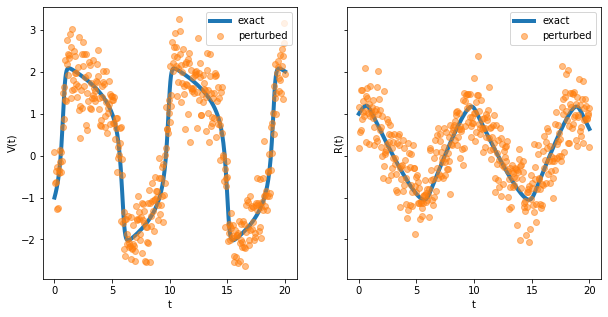
As a final example, we consider the inverse problem of estimating the parameters from noisy solutions of the FitzHugh-Nagumo model.
a = 0.2
b = 0.2
c = 3.0
V_0 = -1.0
R_0 = 1
def fitz_hugh(y, t, a, b, c):
    V, R = y
    return [
        c * (V - V**3 / 3 + R),
        - 1 / c * (V - a - b * R)
    ]
from scipy.integrate import odeint
t = np.linspace(0.0, 20.0, 401)
exact = odeint(fitz_hugh, [V_0, R_0], t, args=(a, b, c))
perturbed = exact + 0.5 * np.random.randn(*exact.shape)
fig, axes = plt.subplots(figsize=(10, 5), ncols=2, sharey=True)
for i in range(2):
    axes[i].plot(t, sol[:, i], linewidth=4, label='exact')
    axes[i].plot(t, perturbed[:, i], 'o', alpha=0.5, label='perturbed')
    axes[i].set_xlabel('t')
    axes[i].legend()
axes[0].set_ylabel('V(t)')
axes[1].set_ylabel('R(t)');
def fitz_hugh_approx(params):
    a, b, c, V_0, R_0 = params
    approx = odeint(fitz_hugh, [V_0, R_0], t, args=(a, b, c))
    return -np.linalg.norm(approx - exact)
np.random.seed(1234)
µ_0 = np.array([0.0, 0.0, 5.0, 0.0, 0.0])
σ_0 = np.array([1.0, 1.0, 1.0, 1.0, 1.0])
opt_x, opt_value, history = cem(fitz_hugh_approx, µ_0, σ_0, num_samples=400, rarity=0.1,
                                max_iters=100, omega=0.9, bounds=None)
print(f'# iterations:', len(history))
print(f'optimal value = {opt_value:.4f}')
# iterations: 24
optimal value = -0.5417
fitted = odeint(fitz_hugh, opt_x[3:5], t, args=tuple(opt_x[:3]))
fig, axes = plt.subplots(figsize=(10, 5), ncols=2, sharey=True)
for i in range(2):
    axes[i].plot(t, exact[:, i], linewidth=4, label='exact')
    axes[i].plot(t, fitted[:, i], 'o', alpha=0.25, label='fitted')
    axes[i].set_xlabel('t')
    axes[i].legend()
axes[0].set_ylabel('V(t)')
axes[1].set_ylabel('R(t)');
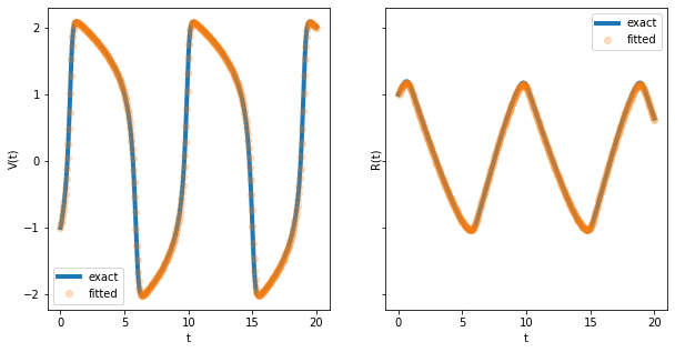
To conclude, the cross-entropy method is a robust and versatile optimizer that deserves to be in every optimization toolbox. In its basic form it is easy to code and only has a few parameters to tune.