In this article we price European options under a two-regime model designed to capture the risk of a currency depeg event. We use the Hong Kong dollar (HKD) as the running example: since 1983 the Hong Kong Monetary Authority (HKMA) has maintained the USD/HKD exchange rate within the band $[7.75, 7.85]$ under the Linked Exchange Rate System (LERS), intervening at both the strong-side ($7.75$) and weak-side ($7.85$) convertibility undertakings. The model treats the spot process as a reflected geometric Brownian motion inside the band; at a random depeg time it jumps and then transitions permanently to a free-floating regime.
Model Description
Let $S(t)$ denote the asset price and let $\tau$ be the depeg time. We define two regimes.
Regime 0 — Pegged (before depeg)
While $t < \tau$ the spot follows a geometric Brownian motion reflected (in log-space) at the band boundaries $[L, U]$:
\[\frac{dS(t)}{S(t)} = (r - q - \lambda\kappa)\,dt + \sigma_0\,dW(t) + d\Phi^L(t) - d\Phi^U(t), \qquad S(t) \in [L, U],\]where $\sigma_0 > 0$ is the volatility inside the band, $W(t)$ is a Wiener process under the risk-neutral measure, $\Phi^L$, $\Phi^U$ are non-decreasing local-time processes that act only when $\log S(t)$ touches $\log L$ or $\log U$ respectively, keeping the process inside the band, and
\[\kappa = \mathbb{E}\!\left[e^{\mu_J + \sigma_J Z}\right] - 1 = e^{\mu_J + \frac{1}{2}\sigma_J^2} - 1\]is the expected proportional jump size. The term $-\lambda\kappa$ is the jump compensator: it subtracts, at each instant, the expected instantaneous contribution of the depeg jump to $dS/S$, so that the jump does not create a systematic drift.
Why the compensator has the same form as in the Merton jump-diffusion model, despite there being only one jump. In the Merton model the jump process $N_t$ is a Poisson process (intensity $\lambda$, infinitely many jumps); here $N_t = \mathbf{1}_{t \ge \tau}$ fires exactly once. Nevertheless, the local dynamics before the jump are identical. At any time $t < \tau$, the memoryless property of the exponential distribution gives
\[\mathbb{P}(\text{jump in } [t,\, t+dt] \mid \tau > t) = \lambda\,dt + o(dt),\]so the expected drift contribution from the jump per unit time is $\lambda\,\mathbb{E}[e^J - 1]\,S(t)\,dt = \lambda\kappa\,S(t)\,dt$, exactly as in Merton. The compensator $-\lambda\kappa$ is determined by the hazard rate of the jump arrival, not by how many jumps will occur in total.
What does differ is the accumulated compensation over $[0, T]$. By the Doob–Meyer decomposition for a 0-1 counting process with intensity $\lambda$, the compensator of $N_t$ is $\lambda(t \wedge \tau)$, not $\lambda t$: the process $N_t - \lambda(t \wedge \tau)$ is a martingale. Consequently the total drift subtracted over the life of the option is
\[\lambda\kappa\,\mathbb{E}[\min(\tau, T)] = \kappa\bigl(1 - e^{-\lambda T}\bigr) \quad \text{vs.} \quad \lambda\kappa T \;\text{(Merton)}.\]The $\lambda$ cancels because $\mathbb{E}[\min(\tau, T)] = \int_0^T e^{-\lambda t}\,dt = (1 - e^{-\lambda T})/\lambda$: a higher intensity means the compensator is applied at a faster rate but for a shorter expected duration, and the two effects offset exactly. What remains is $\kappa$ scaled by the probability that the depeg has occurred by $T$.
In the depeg model the compensation stops after $\tau$ because Regime 1 carries no further jump risk; the SDE self-consistently switches off the $-\lambda\kappa$ term once $t \ge \tau$.
Equivalently, setting $x(t) = \log S(t)$, the log-price satisfies
\[dx(t) = \Bigl(r - q - \lambda\kappa - \tfrac{1}{2}\sigma_0^2\Bigr)\,dt + \sigma_0\,dW(t) + d\tilde{\Phi}^L(t) - d\tilde{\Phi}^U(t), \qquad x(t) \in [\log L,\, \log U],\]where $\tilde{\Phi}^L = \Phi^L / L$ and $\tilde{\Phi}^U = \Phi^U / U$ are the rescaled local times in log-space (the factors $1/L$ and $1/U$ arise from the chain rule $d(\log S) = dS/S$, evaluated at $S = L$ and $S = U$ respectively). This is an arithmetic reflected BM on the log-price interval $[\log L, \log U]$.
Regime 1 — Free-floating (after depeg)
Once $t \ge \tau$ the peg is broken and the spot follows a standard geometric Brownian motion:
\[\frac{dS(t)}{S(t)} = (r - q)\,dt + \sigma_1\,dW(t), \qquad S(t) > 0,\]where $r$ is the HKD risk-free rate, $q$ is the USD risk-free rate, and $\sigma_1 > 0$ is the post-depeg volatility.
Switching Mechanism and Depeg Jump
The depeg time $\tau$ is modelled as the first arrival time of a Poisson process with constant intensity $\lambda > 0$, independent of $W$:
\[\tau \sim \operatorname{Exp}(\lambda), \qquad \mathbb{P}(\tau > t) = e^{-\lambda t}.\]At the moment of the depeg the spot jumps by a random log-normal factor before entering the free-floating regime:
\[S(\tau^+) = S(\tau^-) \cdot e^{\mu_J + \sigma_J Z}, \qquad Z \sim \mathcal{N}(0,1) \text{ independent of everything else.}\]The parameter $\mu_J$ encodes the expected direction of the move and $\sigma_J$ captures uncertainty around the jump size. The transition is permanent: once the process enters Regime 1 it never returns to Regime 0.
Assumptions
- Interest rates $r$, $q$, volatilities $\sigma_0$, $\sigma_1$, the band boundaries $L < U$, and the parameters $\lambda$, $\mu_J$, $\sigma_J$ are all constant.
- The option has a European payoff $\varphi(S(T))$ at maturity $T$; we use a call, $\varphi(S) = (S - K)^+$, as the running example.
- The initial spot satisfies $S(0) = S_0 \in [L, U]$, i.e. we start in Regime 0.
- The jump compensator $-\lambda\kappa$ makes the discounted spot $e^{-(r-q)t}S(t)$ a local martingale globally across both regimes. Because the reflected boundaries create an asymmetric local-time push (see the Forward Price section), the true forward $\mathbb{E}^Q[S(T)]$ differs slightly from the cost-of-carry formula $S_0 e^{(r-q)T}$ and is computed numerically.
- No transaction costs.
Forward Price
A forward contract with delivery price $K$ pays $S(T) - K$ at maturity $T$. Under risk-neutral pricing, its value today is
\[V(0) = e^{-rT}\,\mathbb{E}^Q[S(T) - K] = e^{-rT}\!\left(\mathbb{E}^Q[S(T)] - K\right).\]Step 1 — Express the forward price as an expectation. The delivery price that makes $V(0) = 0$ is
\[F = \mathbb{E}^Q[S(T)].\]Step 2 — Introduce the discount factor. Multiply and divide by $e^{(r-q)T}$:
\[F = e^{(r-q)T}\,\mathbb{E}^Q\!\left[e^{-(r-q)T}S(T)\right].\]It therefore suffices to evaluate $\mathbb{E}^Q[M_T]$, where $M_t = e^{-(r-q)t}S(t)$ is the discounted spot.
Step 3 — Show that $M_t$ has zero drift. In Regime 0, with the jump compensator included in the drift, $M_t$ satisfies
\[dM_t = \underbrace{-\lambda\kappa\,M_t\,dt}_{\text{compensated drift}} + \sigma_0\,M_t\,dW_t + M_t\,d\tilde\Phi_t + \underbrace{M_{t^-}(e^J - 1)\,dN_t}_{\text{single jump at }\tau},\]where $N_t = \mathbf{1}_{t \ge \tau}$ is the depeg indicator, $d\tilde\Phi_t = d\tilde\Phi^L_t - d\tilde\Phi^U_t$ collects the boundary local times, and $J = \mu_J + \sigma_J Z$. The absolutely continuous (i.e. $dt$) part of the drift receives exactly two contributions:
| Source | Contribution to $dt$-drift |
|---|---|
| Regime-0 drift (with compensator) | $-\lambda\kappa\,M_t\,dt$ |
| Expected jump at Poisson rate $\lambda$ | $+\lambda\,\mathbb{E}[e^J - 1]\,M_t\,dt = +\lambda\kappa\,M_t\,dt$ |
| Boundary local times $d\tilde\Phi$ | $0\,dt$ (singular w.r.t.\ Lebesgue measure, zero $dt$-component) |
The first two cancel exactly:
\[-\lambda\kappa\,M_t + \lambda\kappa\,M_t = 0.\]Hence $M_t$ is a local martingale. After $\tau$, Regime 1 is a standard discounted GBM with zero drift, so the local martingale property continues to hold.
Step 4 — Boundary correction. Although the local times have zero $dt$-component, their contribution to $\mathbb{E}[M_T] - M_0$ need not vanish:
\[\mathbb{E}[M_T] - M_0 = L\,\mathbb{E}\!\left[\int_0^T e^{-(r-q)t}\,d\tilde\Phi^L_t\right] - U\,\mathbb{E}\!\left[\int_0^T e^{-(r-q)t}\,d\tilde\Phi^U_t\right].\]In the stationary limit, local-time at boundary $b$ accumulates at rate $\tfrac{\sigma_0^2}{2}\pi(b)$, so the correction is proportional to $L\pi(\ell) - U\pi(u)$. With the stationary density $\pi(y) \propto e^{2\alpha(y-\ell)}$ this equals zero only when $\alpha = -\tfrac{1}{2}$, i.e.\ when $r - q = \lambda\kappa$ exactly.
For the HKD parameters $\alpha \approx 11.6$ and band width $W = \log(U/L) \approx 0.013$, so $U\pi(u) / L\pi(\ell) = (U/L)\,e^{2\alpha W} \approx 1.38$, and the correction is approximately $-1.6\%$:
\[F_{\rm model} = \mathbb{E}^Q[S(T)] \approx 0.984\;S_0\,e^{(r-q)T}.\]We compute $F_{\rm model}$ numerically from the Regime-0 density in the Implied Volatility section below. The pricing formula for European options remains exact — it is derived directly from the path decomposition and does not assume $F = S_0 e^{(r-q)T}$.
Remark. The cost-of-carry formula $F = S_0 e^{(r-q)T}$ is recovered whenever the boundary correction vanishes, which happens for example when $L = U$ (no band), when $\alpha = 0$ (symmetric band with $r - q = \lambda\kappa$), or in the limit $W \to 0$. The band width for HKD is only $\approx 1.3\%$, so the correction is small in absolute terms even though $\alpha$ is large.
Vanilla Option Price
We price a European call with strike $K$ and maturity $T$. The put price follows from put-call parity. The risk-neutral price is
\[C(S_0, T; K) = e^{-rT}\,\mathbb{E}^Q\!\left[(S(T) - K)^+\right].\]Step 1 — Split on the depeg event. By the law of total expectation, partition on whether the depeg has occurred by $T$:
\[C = \underbrace{e^{-rT}\,\mathbb{E}^Q\!\left[(S(T)-K)^+\,\mathbf{1}_{\tau > T}\right]}_{C_{\rm peg}} + \underbrace{e^{-rT}\,\mathbb{E}^Q\!\left[(S(T)-K)^+\,\mathbf{1}_{\tau \le T}\right]}_{C_{\rm dep}}.\]Step 2 — No-depeg term $C_{\rm peg}$. Since $\tau$ is independent of $W$, the indicator $\mathbf{1}_{\tau > T}$ and the Regime-0 path are independent:
\[C_{\rm peg} = \mathbb{P}(\tau > T)\cdot e^{-rT}\,\mathbb{E}^Q_0\!\left[(S^{(0)}(T)-K)^+\right] = e^{-(\lambda + r)T}\!\int_L^U (x-K)^+\,p_0^*(T;\,S_0,\,x)\,dx,\]where $p_0^*(T; S_0, x)$ is the transition density of the Regime-0 reflected GBM (drift $r - q - \lambda\kappa$, vol $\sigma_0$, band $[L,U]$), derived below. Since $S^{(0)}(T) \in [L, U]$ always, this term vanishes for $K \ge U$.
Step 3 — Depeg term $C_{\rm dep}$: closed form conditional on $(\tau, S(\tau^-))$. Conditioning on the depeg time $\tau = s$, whose density is $\lambda e^{-\lambda s}$:
\[C_{\rm dep} = \int_0^T \lambda e^{-\lambda s}\, e^{-rT}\,\mathbb{E}^Q\!\left[(S(T)-K)^+\,\big|\,\tau = s\right]ds.\]Fix $\tau = s$ and $S(s^-) = x$. The terminal price is the product of three independent factors:
\[S(T) = \underbrace{x}_{\text{pre-depeg}} \cdot \underbrace{e^{\,\mu_J + \sigma_J Z}}_{\text{jump at }\tau} \cdot \underbrace{e^{(r-q-\frac{1}{2}\sigma_1^2)(T-s)\,+\,\sigma_1\sqrt{T-s}\,\tilde{Z}}}_{\text{Regime-1 GBM}},\]with $Z, \tilde{Z} \overset{\rm iid}{\sim} \mathcal{N}(0,1)$ independent of everything else. Taking the log:
\[\log S(T)\,\big|\,(\tau=s,\,S(s^-)=x)\;\sim\;\mathcal{N}\!\left(\log x + \mu_J + \left(r - q - \tfrac{\sigma_1^2}{2}\right)(T-s),\;\; \tilde{\sigma}^2(s)\right),\]where the total variance $\tilde{\sigma}^2(s) = \sigma_J^2 + \sigma_1^2(T-s)$ accumulates jump-size uncertainty and post-depeg diffusion. For a log-normal $Y$ with $\log Y \sim \mathcal{N}(m, v^2)$ the discounted call is $e^{-r\tau}\mathbb{E}[(Y-K)^+] = e^{m + v^2/2 - r\tau}N(d_+) - Ke^{-r\tau}N(d_-)$ with $d_\pm = (m + v^2 - \log K \pm 0)/v$. Applying this with $v = \tilde{\sigma}(s)$:
\[e^{m + \tilde{\sigma}^2(s)/2} = x\,e^{\mu_J + \frac{1}{2}\sigma_J^2+(r-q)(T-s)} = x(1+\kappa)\,e^{(r-q)(T-s)},\]so the discounted conditional call price is
\[V^J(x,\,s) \;:=\; e^{-r(T-s)}\,\mathbb{E}^Q\!\left[(S(T)-K)^+\,\big|\,\tau=s,\,S(s^-)=x\right] = x(1+\kappa)\,e^{-q(T-s)}\,N\!\left(\hat{d}_1\right) - K\,e^{-r(T-s)}\,N\!\left(\hat{d}_2\right),\] \[\hat{d}_1(x,s) = \frac{\log\dfrac{x(1+\kappa)}{K} + (r-q)(T-s) + \tfrac{1}{2}\tilde{\sigma}^2(s)}{\tilde{\sigma}(s)}, \qquad \hat{d}_2 = \hat{d}_1 - \tilde{\sigma}(s), \qquad \tilde{\sigma}(s) = \sqrt{\sigma_J^2 + \sigma_1^2(T-s)}.\]This is a Black-Scholes formula with two modifications:
| Standard BS | This model |
|---|---|
| Spot $x$ | Effective spot $x(1+\kappa)$: pre-depeg level scaled by the mean jump |
| Vol $\sigma_1\sqrt{T-s}$ | Total vol $\tilde{\sigma}(s) = \sqrt{\sigma_J^2 + \sigma_1^2(T-s)}$: jump uncertainty adds to diffusive variance |
When $\sigma_J \to 0$ (deterministic jump), $\tilde{\sigma}(s) \to \sigma_1\sqrt{T-s}$ and $V^J$ reduces to the standard BS formula at the shifted spot $x(1+\kappa)$.
Step 4 — Depeg term $C_{\rm dep}$: integrate over the pre-depeg distribution. Since $S(s^-)$ follows the Regime-0 reflected GBM, its density at time $s$ is $p_0^*(s; S_0, x)$. Averaging over $x$ and then over $s$:
\[C_{\rm dep} = \int_0^T \lambda\,e^{-(\lambda + r)s}\!\int_L^U p_0^*(s;\,S_0,\,x)\,V^J(x,\,s)\,dx\;ds.\]Full pricing formula. Combining Steps 2 and 4:
\[\boxed{C(S_0,T;K) \;=\; e^{-(\lambda+r)T}\!\int_L^U (x-K)^+\,p_0^*(T;\,S_0,x)\,dx \;+\; \int_0^T\!\lambda\, e^{-(\lambda+r)s}\!\int_L^U p_0^*(s;\,S_0,\,x)\,V^J(x,s)\,dx\;ds.}\]Both integrals share a single ingredient: $p_0^*$, the Regime-0 transition density, derived next. Put-call parity $P - C = Ke^{-rT} - S_0e^{-qT}$ gives the put price for free.
Regime-0 transition density $p_0^*$
In log-space, $X(t) = \log S(t)$ is an arithmetic BM with drift $\mu^* = r - q - \lambda\kappa - \tfrac{1}{2}\sigma_0^2$ and vol $\sigma_0$, reflected at $\ell = \log L$ and $u = \log U$. Its transition density $\tilde{p}_0^*(t;\,x_0,\,y)$ satisfies the Fokker-Planck PDE
\[\partial_t \tilde{p} = \tfrac{\sigma_0^2}{2}\,\partial_{yy}\tilde{p} - \mu^*\,\partial_y\tilde{p}, \qquad y \in (\ell, u),\]with no-flux (reflecting) boundary conditions at both ends:
\[\Bigl(\mu^*\tilde{p} - \tfrac{\sigma_0^2}{2}\,\partial_y\tilde{p}\Bigr)\Big|_{y=\ell,\,u} = 0.\]Removing the drift. Substitute $\tilde{p}(t;\,x_0,\,y) = e^{\,\alpha y - \frac{\alpha^2\sigma_0^2}{2}t}\,g(t;\,x_0,\,y)$, where $\alpha = \mu^*/\sigma_0^2$. Inserting into the PDE shows that all $\alpha$-dependent terms cancel, leaving $g$ satisfying the heat equation:
\[\partial_t g = \tfrac{\sigma_0^2}{2}\,\partial_{yy}g.\]Substituting the same ansatz into the no-flux BCs and simplifying (using $\mu^* = \alpha\sigma_0^2$) yields Robin boundary conditions for $g$:
\[\partial_y g\big|_{y=\ell,\,u} = \alpha\, g\big|_{y=\ell,\,u}.\]Eigenfunction expansion. The eigenvalue problem $g’’ = -\beta^2 g$ with Robin BCs $g’(\ell) = \alpha g(\ell)$, $g’(u) = \alpha g(u)$ is solved by $\beta_n = n\pi/(u-\ell)$, $n \ge 1$, with eigenfunctions
\[\Phi_n(y) = \cos\!\left(\frac{n\pi(y-\ell)}{u-\ell}\right) + \frac{\alpha(u-\ell)}{n\pi}\,\sin\!\left(\frac{n\pi(y-\ell)}{u-\ell}\right), \qquad \|\Phi_n\|^2 = \frac{u-\ell}{2}\!\left(1 + \frac{\alpha^2(u-\ell)^2}{n^2\pi^2}\right).\]The sine term is a correction of order $\alpha(u-\ell)/(n\pi)$ relative to the cosine; for the HKD parameters this is $\approx 5\%$ for $n=1$ and negligible for large $n$. The Robin problem also admits a growing mode $g_0(y) = e^{\alpha(y-\ell)}$; after back-substituting via the $e^{\alpha y}$ factor it contributes a $t$-independent term that equals the stationary distribution $\pi(y) \propto e^{2\alpha(y-\ell)}$. Expanding $g$ in the full basis and summing:
\[\tilde{p}_0^*(t;\,x_0,\,y) = \underbrace{\frac{2\alpha\,e^{2\alpha(y-\ell)}}{e^{2\alpha(u-\ell)}-1}}_{\pi(y),\;\text{stationary}} + e^{\,\alpha(y-x_0)}\sum_{n=1}^{\infty} \frac{2\beta_n^2\,e^{-\frac{\sigma_0^2(\alpha^2+\beta_n^2)}{2}t}}{(u-\ell)(\alpha^2+\beta_n^2)}\,\Phi_n(x_0)\,\Phi_n(y), \qquad \beta_n = \frac{n\pi}{u-\ell}.\]The asset-space density follows by the change of variables $x = e^y$:
\[p_0^*(t;\,S_0,\,x) = \frac{1}{x}\,\tilde{p}_0^*\!\left(t;\;\log S_0,\;\log x\right), \qquad x \in [L, U].\]The series decays as $e^{-\sigma_0^2\beta_n^2 t/2}$ and converges rapidly once $t \gtrsim (u-\ell)^2/(\pi^2\sigma_0^2)$. For small $t$ (spot far from the boundaries) the density is well approximated by a Gaussian.
Monte Carlo Simulation
Before evaluating the semi-analytic formula we build a Monte Carlo pricer to develop intuition and serve as a reference. Each path is simulated as follows:
- Draw $\tau \sim \operatorname{Exp}(\lambda)$ independently for each path.
- While $t < \tau$, advance the log-price using the jump-compensated Euler–Maruyama step for the reflected arithmetic BM: \(x_{i+1} = \operatorname{reflect}\!\left(x_i + \underbrace{\bigl(r - q - \lambda\kappa - \tfrac{1}{2}\sigma_0^2\bigr)\Delta t}_{\text{compensated Itô drift}} + \sigma_0\sqrt{\Delta t}\,Z_i,\; \log L,\; \log U\right).\)
- At the first grid time $t_i \ge \tau$, apply the log-normal jump: $x \leftarrow x + \mu_J + \sigma_J Z’$, $Z’ \sim \mathcal{N}(0,1)$.
- For $t \ge \tau$, advance as standard GBM in Regime 1: $x_{i+1} = x_i + (r - q - \tfrac{1}{2}\sigma_1^2)\Delta t + \sigma_1\sqrt{\Delta t}\,Z_i$.
The reflection in Step 2 is handled by the triangle-wave identity, which folds any value back into $[\log L, \log U]$ and correctly handles multiple boundary crossings within a single step. Applying the jump at the nearest grid point (Step 3) instead of exactly at $\tau$ introduces an $O(\Delta t)$ discretization error; at 252 steps per year this is negligible.
from collections import namedtuple
import matplotlib.patches as mpatches
import matplotlib.pylab as plt
import numpy as np
Model = namedtuple('Model', ['S0', 'L', 'U', 'sigma0', 'r', 'q', 'sigma1', 'lam', 'T', 'mu_J', 'sigma_J'])

model = Model(
    S0=7.78,      # USD/HKD spot (typical 2024 level)
    L=7.75,       # HKMA strong-side convertibility undertaking
    U=7.85,       # HKMA weak-side convertibility undertaking
    sigma0=0.02,  # lognormal vol inside band (annualised)
    r=0.05,       # HKD risk-free rate
    q=0.04,       # USD risk-free rate
    sigma1=0.08,  # GBM vol post-depeg (annualised)
    lam=0.10,     # depeg intensity: ~10% annual probability
    T=1.0,        # option maturity in years
    mu_J=0.05,    # log-mean jump at depeg
    sigma_J=0.03, # uncertainty around the jump size
)
Path Simulation
In Regime 0 we simulate the log-price $x(t) = \log S(t)$, which follows an arithmetic reflected BM on $[\log L, \log U]$ with jump-compensated Ito drift $(r - q - \lambda\kappa - \frac{1}{2}\sigma_0^2)$, where $\kappa = e^{\mu_J + \frac{1}{2}\sigma_J^2} - 1$. The reflection map folds any value outside the interval back inside by mirroring at the boundaries — it is the triangle wave with period $2(\log U - \log L)$:
\[\operatorname{reflect}(x;\, \ell, u) = \ell + \left| \bigl((x - \ell) \bmod 2(u - \ell)\bigr) - (u - \ell) \right|.\]Applied with $\ell = \log L$ and $u = \log U$, this keeps $x(t) \in [\log L, \log U]$, so $S(t) = e^{x(t)} \in [L, U]$ automatically.
def reflect(x, lo, hi):
    width = hi - lo
    z = (x - lo) % (2 * width)
    return lo + np.where(z <= width, z, 2 * width - z)


def simulate_paths(model, num_paths, num_steps, rng):
    dt = model.T / num_steps
    sqrt_dt = np.sqrt(dt)
    t_grid = np.linspace(0.0, model.T, num_steps + 1)

    log_L = np.log(model.L)
    log_U = np.log(model.U)
    kappa = np.exp(model.mu_J + 0.5 * model.sigma_J ** 2) - 1  # expected proportional jump size
    drift0 = (model.r - model.q - model.lam * kappa - 0.5 * model.sigma0 ** 2) * dt  # jump-compensated Ito drift

    tau = rng.exponential(1.0 / model.lam, size=num_paths)  # depeg times

    # Each path draws one log-jump applied at the single switching moment.
    log_jumps = model.mu_J + model.sigma_J * rng.standard_normal(num_paths)
    jumped    = np.zeros(num_paths, dtype=bool)   # tracks which paths have jumped

    S      = np.empty((num_steps + 1, num_paths))
    S[0]   = model.S0
    log_S  = np.full(num_paths, np.log(model.S0))
    Z      = rng.standard_normal((num_steps, num_paths))

    for i in range(num_steps):
        in_pegged = tau > t_grid[i]

        # Paths entering regime 1 for the first time at this step
        switching_now = ~in_pegged & ~jumped

        # Apply one-time multiplicative jump at the switching moment (in log-space)
        log_S_base = np.where(switching_now, log_S + log_jumps, log_S)
        jumped |= switching_now

        # Regime 0: step log-price with jump-compensated Ito drift, then reflect in log-space
        log_S_new = reflect(
            log_S + drift0 + model.sigma0 * sqrt_dt * Z[i],
            log_L, log_U,
        )
        S_pegged = np.exp(log_S_new)

        # Regime 1: standard GBM from the (possibly jump-adjusted) base
        S_free = np.exp(log_S_base) * np.exp(
            (model.r - model.q - 0.5 * model.sigma1 ** 2) * dt
            + model.sigma1 * sqrt_dt * Z[i]
        )

        S[i + 1] = np.where(in_pegged, S_pegged, S_free)
        log_S = np.where(in_pegged, log_S_new, np.log(S_free))

    return t_grid, S, tau
Path Visualisation
We simulate 100 paths and colour each segment by regime: blue while the peg holds, red after the depeg. The shaded strip marks the band $[L, U]$.
rng = np.random.default_rng(42)
num_paths = 100
num_steps = int(252 * model.T)

t_grid, S, tau = simulate_paths(model, num_paths, num_steps, rng)

fig, ax = plt.subplots(figsize=(12, 5))

ax.axhspan(model.L, model.U, color='steelblue', alpha=0.07)
ax.axhline(model.L, color='steelblue', lw=0.9, ls='--', label=f'L = {model.L}')
ax.axhline(model.U, color='steelblue', lw=0.9, ls='--', label=f'U = {model.U}')
ax.axhline(model.S0, color='grey', lw=0.6, ls=':')

for j in range(num_paths):
    i_dep = int(np.searchsorted(t_grid, tau[j]))
    if i_dep <= num_steps:
        ax.plot(t_grid[:i_dep + 1], S[:i_dep + 1, j], color='steelblue', lw=0.5, alpha=0.45)
        ax.plot(t_grid[i_dep:],     S[i_dep:,     j], color='tomato',    lw=0.5, alpha=0.45)
    else:
        ax.plot(t_grid, S[:, j], color='steelblue', lw=0.5, alpha=0.45)

ax.set_xlabel('Time (years)')
ax.set_ylabel('USD/HKD')
ax.set_title('USD/HKD two-regime depeg model — 100 Monte Carlo paths')
ax.legend(handles=[
    mpatches.Patch(color='steelblue', alpha=0.6, label='Regime 0 (pegged)'),
    mpatches.Patch(color='tomato',    alpha=0.6, label='Regime 1 (free-floating)'),
    mpatches.Patch(color='steelblue', alpha=0.15, label=f'HKMA band [{model.L}, {model.U}]'),
], loc='upper left')
plt.tight_layout()
plt.show()

n_dep = (tau <= model.T).sum()
print(f"Paths that depeg before T = {model.T}: {n_dep}/{num_paths} ({100*n_dep/num_paths:.0f}%)")
print(f"Theoretical probability:               {100*(1 - np.exp(-model.lam * model.T)):.0f}%")
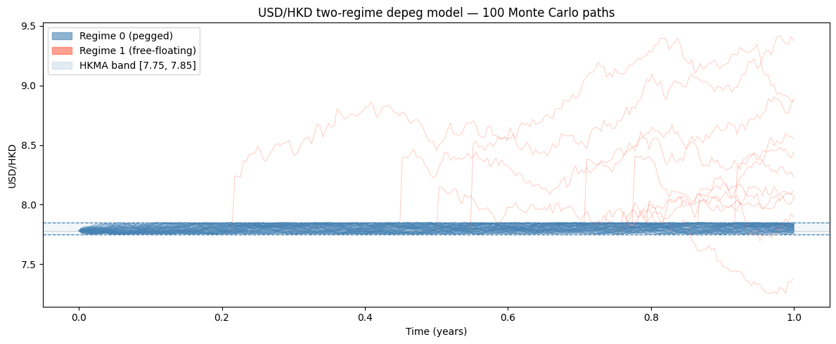
Paths that depeg before T = 1.0: 11/100 (11%)
Theoretical probability:               10%
Numerical Validation
We validate the semi-analytic formula against Monte Carlo in two steps, from simpler to harder:
- Forward price — verify that the analytic $F_{\rm model} = \mathbb{E}^Q[S(T)]$ computed from the density matches the Monte Carlo estimate. This tests that the density series integrates to 1 and that the first moment is accurate before we touch option prices.
- Vanilla call prices — compare the full semi-analytic price against Monte Carlo across a grid of strikes. This tests the $C_{\rm peg}$ and $C_{\rm dep}$ integrals end-to-end.
Semi-analytic pricer. The Regime-0 density $p_0^*(t;\,S_0,\,x)$ is computed via the eigenfunction series (50 terms) on an $80\times 80$ $(s,x)$ grid. The $s$-grid starts at $s_{\min} = 10^{-6}$ years rather than $0$ to capture the finite contribution of early depegs (the integrand converges to $\lambda V^J(S_0,0)$ as $s\to 0$). The density is pre-computed once and shared across both validations and the IV smile.
Monte Carlo. All MC estimates use simulate_paths with 252 steps per year. Confidence intervals are $\pm 1.96\,\hat\sigma/\sqrt{N}$.
from scipy.stats import norm

# ── Regime-0 transition density via eigenfunction expansion ─────────────
def _p0_log_vec(t, x0, y_arr, model, N_terms=50):
    """
    Vectorised Regime-0 log-price transition density tilde_p0*(t; x0, y)
    for y in y_arr (numpy array of log-prices).
    """
    ell = np.log(model.L)
    u   = np.log(model.U)
    width   = u - ell
    kappa   = np.exp(model.mu_J + 0.5 * model.sigma_J**2) - 1
    mu_star = model.r - model.q - model.lam * kappa - 0.5 * model.sigma0**2
    alpha   = mu_star / model.sigma0**2
    y = np.asarray(y_arr, dtype=float)

    # n=0 stationary mode  π(y) ∝ e^{2α(y-ℓ)}, independent of x0
    if np.abs(alpha) < 1e-12:
        stat = np.ones_like(y) / width
    else:
        stat = 2.0 * alpha * np.exp(2.0 * alpha * (y - ell)) / (np.exp(2.0 * alpha * width) - 1.0)

    # n>=1 oscillatory modes
    series = np.zeros_like(y)
    for n in range(1, N_terms + 1):
        beta_n  = n * np.pi / width
        phi_x0  = np.cos(beta_n*(x0 - ell)) + (alpha/beta_n)*np.sin(beta_n*(x0 - ell))
        phi_y   = np.cos(beta_n*(y  - ell)) + (alpha/beta_n)*np.sin(beta_n*(y  - ell))
        coeff   = 2.0 * beta_n**2 / (width * (alpha**2 + beta_n**2))
        decay   = np.exp(-0.5 * model.sigma0**2 * (alpha**2 + beta_n**2) * t)
        series += coeff * decay * phi_x0 * phi_y

    return stat + np.exp(alpha * (y - x0)) * series


# ── Pre-compute density on an (s, x) grid — shared across all sections ───
N_TERMS, NX, NS = 50, 80, 80
x_grid  = np.linspace(model.L, model.U, NX)
s_grid  = np.linspace(1e-6, model.T, NS)   # start near 0, not at T/N
log_x0  = np.log(model.S0)
log_x   = np.log(x_grid)
kappa_v = np.exp(model.mu_J + 0.5 * model.sigma_J**2) - 1

print("Pre-computing Regime-0 density on (s, x) grid …", end="  ", flush=True)
p0_grid = np.stack([_p0_log_vec(s, log_x0, log_x, model, N_TERMS) / x_grid
                    for s in s_grid])         # shape (NS, NX), p0*(s; S0, x)
p0_at_T = _p0_log_vec(model.T, log_x0, log_x, model, N_TERMS) / x_grid   # shape (NX,)
print("done.")


# ── Semi-analytic call (uses the pre-computed density) ───────────────────
def semi_analytic_call(K):
    # C_peg: no-depeg term
    C_peg = (np.exp(-(model.lam + model.r) * model.T)
             * np.trapezoid(np.maximum(x_grid - K, 0.0) * p0_at_T, x_grid))

    # V^J on the full (NS, NX) grid
    tau_rem   = (model.T - s_grid)[:, None]          # (NS, 1)
    sig_tilde = np.sqrt(model.sigma_J**2 + model.sigma1**2 * tau_rem)
    eff_spot  = x_grid[None, :] * (1.0 + kappa_v)   # (1, NX)
    d1 = (np.log(eff_spot / K) + (model.r - model.q)*tau_rem + 0.5*sig_tilde**2) / sig_tilde
    d2 = d1 - sig_tilde
    vj = (eff_spot * np.exp(-model.q * tau_rem) * norm.cdf(d1)
          - K      * np.exp(-model.r * tau_rem) * norm.cdf(d2))

    # C_dep: outer integral over s
    weight = model.lam * np.exp(-(model.lam + model.r) * s_grid)   # (NS,)
    C_dep  = np.trapezoid(weight * np.trapezoid(p0_grid * vj, x_grid, axis=1), s_grid)

    return C_peg + C_dep
Pre-computing Regime-0 density on (s, x) grid … done.
Forward Price
We first verify that $F_{\rm model} = \mathbb{E}^Q[S(T)]$ computed analytically from the density matches the Monte Carlo estimate. We also decompose the forward into the no-depeg and depeg contributions:
-
No-depeg paths ($\tau > T$, probability $e^{-\lambda T} \approx 60.6\%$): $S(T) \in [L, U]$, so $\mathbb{E}[S(T)\, \,\tau > T]$ must lie in $[7.75, 7.85]$. -
Depeg paths ($\tau \le T$, probability $\approx 39.4\%$): after the upward jump, $\mathbb{E}[S(T)\, \,\tau \le T]$ sits well above the band.
# ── Model-consistent forward E[S(T)] from the density ────────────────────
# p0_grid[i, j] = p0*(s_i; S0, x_j)  →  E[S(s)] = ∫ x·p0*(s;S0,x) dx
m1_s = np.trapezoid(x_grid * p0_grid, x_grid, axis=1)   # shape (NS,)
m1_T = np.trapezoid(x_grid * p0_at_T, x_grid)           # scalar

# E[S(T)] = e^{-λT}·E[S(T)|no depeg]
#          + ∫₀ᵀ λe^{-λs}·(1+κ)·e^{(r-q)(T-s)}·E[S(s)|regime 0] ds
F_model = (
    np.exp(-model.lam * model.T) * m1_T
    + np.trapezoid(
        model.lam * np.exp(-model.lam * s_grid)
        * (1.0 + kappa_v) * np.exp((model.r - model.q) * (model.T - s_grid))
        * m1_s,
        s_grid,
    )
)
F_bs = model.S0 * np.exp((model.r - model.q) * model.T)

# ── Monte Carlo forward with regime decomposition ─────────────────────────
NUM_PATHS_FWD = 200_000

print(f"Simulating {NUM_PATHS_FWD:,} paths for forward validation …", end="  ", flush=True)
_, S_fwd, tau_fwd = simulate_paths(model, NUM_PATHS_FWD, int(252 * model.T),
                                   np.random.default_rng(99))
S_T_fwd = S_fwd[-1]
print("done.\n")

no_depeg = tau_fwd > model.T
depegged = ~no_depeg

fwd_mc = S_T_fwd.mean()
fwd_se = S_T_fwd.std(ddof=1) / np.sqrt(NUM_PATHS_FWD)

print(f"{'Quantity':<42}  {'Value':>10}")
print("─" * 56)
print(f"{'F_model  (analytic from density)':<42}  {F_model:10.5f}")
print(f"{'E[S(T)]  Monte Carlo':<42}  {fwd_mc:10.5f}")
print(f"{'  95% CI':<42}  [{fwd_mc - 1.96*fwd_se:.5f}, {fwd_mc + 1.96*fwd_se:.5f}]")
print(f"{'F_bs     S0·e^(r-q)T  (cost-of-carry)':<42}  {F_bs:10.5f}")
print()
print(f"{'P(no depeg)  Monte Carlo':<42}  {no_depeg.mean():10.4%}")
print(f"{'P(no depeg)  theory  e^(-λT)':<42}  {np.exp(-model.lam * model.T):10.4%}")
print()
print(f"{'E[S(T) | no depeg]  Monte Carlo':<42}  {S_T_fwd[no_depeg].mean():10.5f}  ← in [{model.L}, {model.U}]")
print(f"{'E[S(T) | depeg]     Monte Carlo':<42}  {S_T_fwd[depegged].mean():10.5f}")

z = (F_model - fwd_mc) / fwd_se
print(f"\nz-score  (F_model − MC) / SE  =  {z:.2f}  (|z| < 1.96 → within 95% CI)")
Simulating 200,000 paths for forward validation …  done.

Quantity                                         Value
────────────────────────────────────────────────────────
F_model  (analytic from density)               7.84455
E[S(T)]  Monte Carlo                           7.84385
  95% CI                                    [7.84293, 7.84477]
F_bs     S0·e^(r-q)T  (cost-of-carry)          7.85819

P(no depeg)  Monte Carlo                      90.5230%
P(no depeg)  theory  e^(-λT)                  90.4837%

E[S(T) | no depeg]  Monte Carlo                7.80221  ← in [7.75, 7.85]
E[S(T) | depeg]     Monte Carlo                8.24156

z-score  (F_model − MC) / SE  =  1.49  (|z| < 1.96 → within 95% CI)
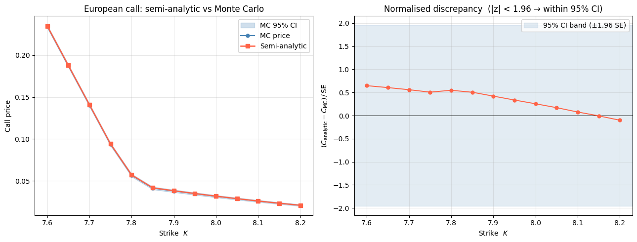
Vanilla Call Prices
We now compare the full semi-analytic call price against Monte Carlo across a grid of strikes $K \in [7.60, 8.20]$ using 50,000 paths. The right panel shows the normalised discrepancy $(C_{\rm analytic} - C_{\rm MC})/\mathrm{SE}$: any value within $\pm 1.96$ means the analytic price falls inside the Monte Carlo 95% CI.
K_grid = np.linspace(7.60, 8.20, 13)
print("Computing semi-analytic prices …", end="  ", flush=True)
analytic_prices = np.array([semi_analytic_call(K) for K in K_grid])
print("done.")

NUM_PATHS_VAL = 50_000
print(f"Simulating {NUM_PATHS_VAL:,} paths …", end="  ", flush=True)
_, S_val, _ = simulate_paths(model, NUM_PATHS_VAL, int(252 * model.T),
                              np.random.default_rng(0))
S_T  = S_val[-1]
disc = np.exp(-model.r * model.T)
print("done.")

mc_prices = np.empty(len(K_grid))
mc_lo     = np.empty(len(K_grid))
mc_hi     = np.empty(len(K_grid))

for i, K in enumerate(K_grid):
    payoffs      = disc * np.maximum(S_T - K, 0.0)
    mean_p       = payoffs.mean()
    se           = payoffs.std(ddof=1) / np.sqrt(NUM_PATHS_VAL)
    mc_prices[i] = mean_p
    mc_lo[i]     = mean_p - 1.96 * se
    mc_hi[i]     = mean_p + 1.96 * se

# ── Plot ──────────────────────────────────────────────────────────────────
fig, axes = plt.subplots(1, 2, figsize=(13, 5))

ax = axes[0]
ax.fill_between(K_grid, mc_lo, mc_hi, color='steelblue', alpha=0.25, label='MC 95% CI')
ax.plot(K_grid, mc_prices,       'o-', color='steelblue', ms=5, lw=1.4, label='MC price')
ax.plot(K_grid, analytic_prices, 's-', color='tomato',   ms=6, lw=1.8, label='Semi-analytic')
ax.set_xlabel('Strike  $K$'); ax.set_ylabel('Call price')
ax.set_title('European call: semi-analytic vs Monte Carlo')
ax.legend(); ax.grid(alpha=0.3)

se_arr  = (mc_hi - mc_prices) / 1.96
z_score = (analytic_prices - mc_prices) / se_arr

ax = axes[1]
ax.axhspan(-1.96, 1.96, color='steelblue', alpha=0.15, label='95% CI band (±1.96 SE)')
ax.axhline(0, color='k', lw=0.8)
ax.plot(K_grid, z_score, 'o-', color='tomato', ms=5, lw=1.4)
ax.set_xlabel('Strike  $K$')
ax.set_ylabel('$(C_{\\rm analytic} - C_{\\rm MC})\,/\,\\mathrm{SE}$')
ax.set_title('Normalised discrepancy  (|z| < 1.96 → within 95% CI)')
ax.legend(); ax.grid(alpha=0.3)

plt.tight_layout()
plt.show()

print(f"\n{'Strike':>8}  {'Analytic':>10}  {'MC price':>10}  {'MC lo':>8}  {'MC hi':>8}  {'z-score':>8}")
print("─" * 66)
for K, cp, cm, lo, hi, z in zip(K_grid, analytic_prices, mc_prices, mc_lo, mc_hi, z_score):
    flag = "" if abs(z) < 1.96 else "  ← outside 95% CI"
    print(f"{K:8.3f}  {cp:10.5f}  {cm:10.5f}  {lo:8.5f}  {hi:8.5f}  {z:8.2f}{flag}")
Computing semi-analytic prices …  done.
Simulating 50,000 paths …

<>:45: SyntaxWarning: invalid escape sequence '\,'
<>:45: SyntaxWarning: invalid escape sequence '\,'
/var/folders/82/lkpb1cxn4rz7l0xpl7j_d8vm0000gn/T/ipykernel_58759/1377245770.py:45: SyntaxWarning: invalid escape sequence '\,'
  ax.set_ylabel('$(C_{\\rm analytic} - C_{\\rm MC})\,/\,\\mathrm{SE}$')


done.
  Strike    Analytic    MC price     MC lo     MC hi   z-score
──────────────────────────────────────────────────────────────────
   7.600     0.23497     0.23440   0.23268   0.23612      0.65
   7.650     0.18790     0.18737   0.18566   0.18909      0.61
   7.700     0.14093     0.14044   0.13873   0.14215      0.56
   7.750     0.09405     0.09361   0.09190   0.09531      0.51
   7.800     0.05704     0.05657   0.05490   0.05825      0.55
   7.850     0.04164     0.04122   0.03962   0.04283      0.51
   7.900     0.03816     0.03784   0.03632   0.03936      0.42
   7.950     0.03484     0.03459   0.03315   0.03603      0.34
   8.000     0.03167     0.03149   0.03014   0.03285      0.26
   8.050     0.02867     0.02856   0.02728   0.02984      0.17
   8.100     0.02585     0.02580   0.02460   0.02701      0.08
   8.150     0.02321     0.02322   0.02209   0.02435     -0.01
   8.200     0.02076     0.02082   0.01976   0.02188     -0.10
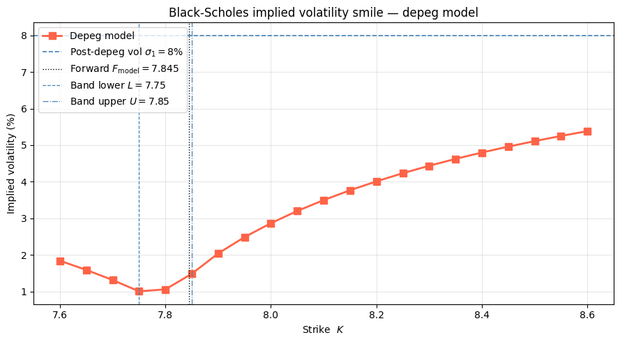
Implied Volatility Smile
A single Black-Scholes model with flat volatility cannot simultaneously price all strikes. We back out the Black-Scholes implied volatility $\hat\sigma(K)$ from each semi-analytic price by inverting the BS formula numerically. The shape of $\hat\sigma(K)$ across strikes is the volatility smile induced by the depeg model.
Because the reflection boundary creates a small downward bias in the model’s forward price (see the Forward Price section), we use the model-consistent forward $F_{\rm model} = \mathbb{E}^Q[S(T)]$ — computed analytically from the Regime-0 density — rather than the cost-of-carry formula $S_0 e^{(r-q)T}$. The implied vol is then defined by inverting the forward-based BS formula
\[C_{\rm BS}(F, K, r, T, \sigma) = e^{-rT}\!\left[F\,N(d_+) - K\,N(d_-)\right], \qquad d_\pm = \frac{\ln(F/K) \pm \tfrac{1}{2}\sigma^2 T}{\sigma\sqrt{T}},\]which is the standard formula with $F = S e^{(r-q)T}$ replaced by $F_{\rm model}$.
The depeg model departs from a flat smile in two characteristic ways:
- Positive skew ($\hat\sigma$ rising with $K$): the jump at depeg is upward-biased ($\mu_J = 0.05 > 0$), making high strikes relatively expensive — they are in-the-money more often after a depeg.
- Level shift above $\sigma_1$: even for strikes well above the band, the implied vol exceeds $\sigma_1 = 8\%$ because jump-size uncertainty $\sigma_J$ adds extra variance at the moment of the peg break.
- Kink near $K = U = 7.85$: for $K < U$ the no-depeg paths contribute positively to the call, boosting the price and compressing the smile; for $K \ge U$ only the depeg paths pay off and the smile steepens sharply.
from scipy.optimize import brentq

# ── Forward-based BS formula and IV inversion ────────────────────────────
def bs_call_fwd(F, K, r, T, sigma):
    """BS call in terms of forward price F (no separate spot/q needed)."""
    sqrtT = np.sqrt(T)
    d1 = (np.log(F / K) + 0.5 * sigma**2 * T) / (sigma * sqrtT)
    d2 = d1 - sigma * sqrtT
    return np.exp(-r * T) * (F * norm.cdf(d1) - K * norm.cdf(d2))


def implied_vol_fwd(price, F, K, r, T, lo=1e-4, hi=5.0):
    """Implied vol relative to forward F; returns NaN when price ≤ intrinsic."""
    intrinsic = max(np.exp(-r * T) * (F - K), 0.0)
    if price <= intrinsic + 1e-10:
        return np.nan
    try:
        return brentq(lambda s: bs_call_fwd(F, K, r, T, s) - price, lo, hi, xtol=1e-9)
    except ValueError:
        return np.nan


# ── Compute IV smile over a wide strike grid ─────────────────────────────
K_iv = np.linspace(7.60, 8.60, 21)

print("Computing semi-analytic prices for IV smile …", end="  ", flush=True)
prices_iv = np.array([semi_analytic_call(K) for K in K_iv])
print("done.")

iv = np.array([implied_vol_fwd(p, F_model, K, model.r, model.T)
               for p, K in zip(prices_iv, K_iv)])


# ── Plot ──────────────────────────────────────────────────────────────────
fig, ax = plt.subplots(figsize=(9, 5))

mask = ~np.isnan(iv)
ax.plot(K_iv[mask], iv[mask] * 100, 's-', color='tomato', ms=7, lw=2.0,
        label='Depeg model')
ax.axhline(model.sigma1 * 100, color='steelblue', lw=1.2, ls='--',
           label=f'Post-depeg vol $\\sigma_1 = {model.sigma1*100:.0f}\\%$')
ax.axvline(F_model, color='black',     lw=1.0, ls=':',
           label=f'Forward $F_ = {F_model:.3f}$')
ax.axvline(model.L, color='steelblue', lw=0.9, ls='--',
           label=f'Band lower $L = {model.L}$')
ax.axvline(model.U, color='steelblue', lw=0.9, ls='-.',
           label=f'Band upper $U = {model.U}$')

ax.set_xlabel('Strike  $K$')
ax.set_ylabel('Implied volatility (%)')
ax.set_title('Black-Scholes implied volatility smile — depeg model')
ax.legend(loc='upper left')
ax.grid(alpha=0.3)
plt.tight_layout()
plt.show()


# ── Summary table ─────────────────────────────────────────────────────────
print(f"\n{'Strike':>8}  {'Model price':>12}  {'Impl. vol':>10}  {'BS flat σ₁':>12}")
print("─" * 48)
for K, p, v in zip(K_iv, prices_iv, iv):
    bs_flat = bs_call_fwd(F_model, K, model.r, model.T, model.sigma1)
    iv_str = f"{v*100:9.2f}%" if not np.isnan(v) else "       NaN"
    print(f"{K:8.3f}  {p:12.5f}  {iv_str}  {bs_flat:12.5f}")
Computing semi-analytic prices for IV smile … done.
  Strike   Model price   Impl. vol    BS flat σ₁
────────────────────────────────────────────────
   7.600       0.23497       1.84%       0.36881
   7.650       0.18790       1.59%       0.33915
   7.700       0.14093       1.31%       0.31099
   7.750       0.09405       1.00%       0.28433
   7.800       0.05704       1.06%       0.25920
   7.850       0.04164       1.48%       0.23559
   7.900       0.03816       2.04%       0.21348
   7.950       0.03484       2.49%       0.19286
   8.000       0.03167       2.87%       0.17370
   8.050       0.02867       3.20%       0.15597
   8.100       0.02585       3.50%       0.13961
   8.150       0.02321       3.77%       0.12458
   8.200       0.02076       4.01%       0.11083
   8.250       0.01850       4.23%       0.09828
   8.300       0.01643       4.44%       0.08689
   8.350       0.01454       4.62%       0.07657
   8.400       0.01282       4.80%       0.06727
   8.450       0.01127       4.96%       0.05892
   8.500       0.00988       5.11%       0.05144
   8.550       0.00864       5.25%       0.04477
   8.600       0.00754       5.38%       0.03885
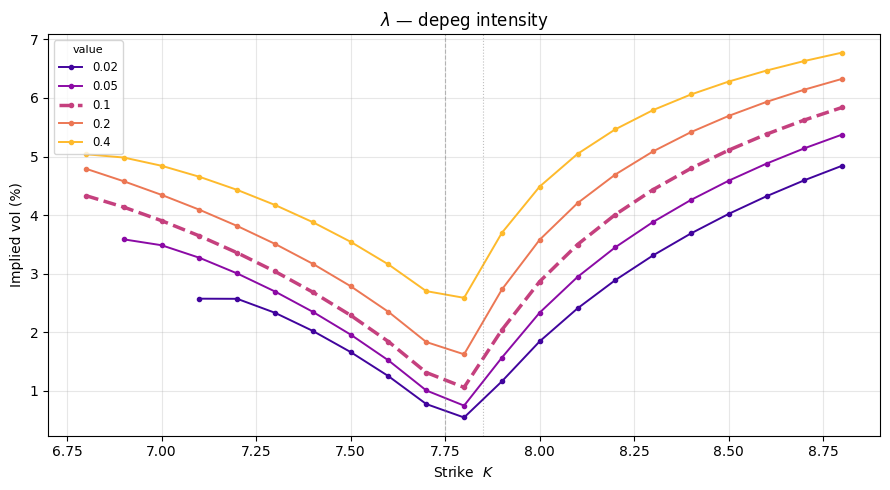
Parameter Sensitivity
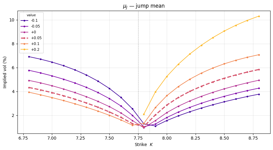
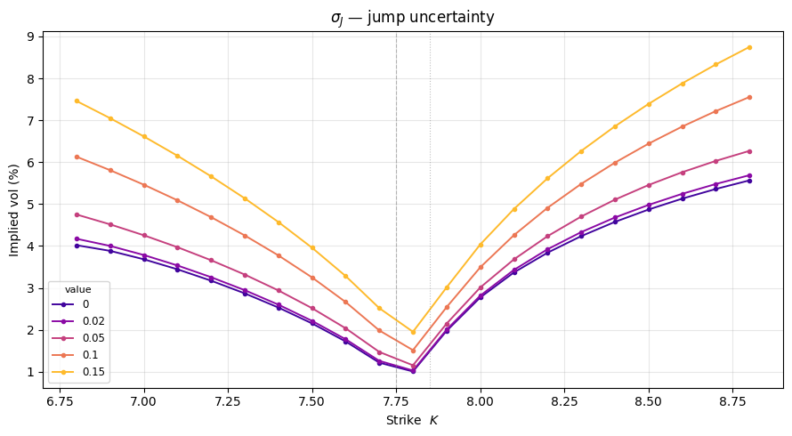
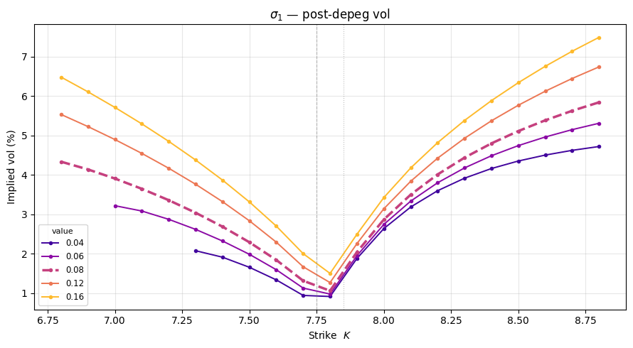
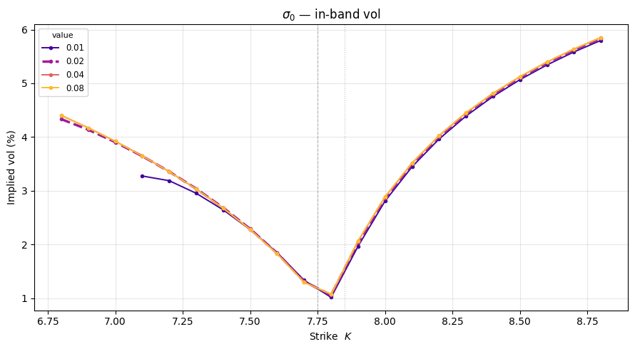
To understand how each parameter shapes the smile, we vary one at a time while holding all others at their baseline values. Each subplot shows a family of IV curves; the thicker dashed line is the baseline.
Key effects to look for:
- $\lambda$ (depeg intensity): scales the overall smile level — higher depeg probability lifts all implied vols proportionally; as $\lambda \to 0$ the smile collapses to a flat line at $\sigma_1$.
- $\mu_J$ (jump mean): controls the skew direction — a positive $\mu_J$ (upward jump) gives a rising smile; negative $\mu_J$ inverts it to a falling smile. The smile pivots around the forward.
- $\sigma_J$ (jump uncertainty): adds a symmetric level shift — it contributes $\sigma_J^2$ of variance at every strike, raising the smile floor independently of $K$.
- $\sigma_1$ (post-depeg vol): shifts the OTM smile rigidly — for $K \gg U$ only post-depeg paths contribute and $\hat\sigma(K) \to \sigma_1$, so this parameter controls the right-wing asymptote.
- $\sigma_0$ (in-band vol): minor effect since the band is narrow ($\approx 1.3\%$); it governs how spread the pre-depeg level $S(\tau^-)$ is across $[L, U]$, which slightly modifies the effective spot entering $V^J$.
# ── Helper: IV smile for an arbitrary model variant ──────────────────────
def compute_smile(mdl, K_grid, N_TERMS=40, NX=60, NS=60):
    """Return (iv_array, F_model) using a fresh density grid for mdl."""
    kv  = np.exp(mdl.mu_J + 0.5 * mdl.sigma_J**2) - 1
    xg  = np.linspace(mdl.L, mdl.U, NX)
    sg  = np.linspace(1e-6, mdl.T, NS)
    lx0 = np.log(mdl.S0)
    lx  = np.log(xg)

    p0g = np.stack([_p0_log_vec(s, lx0, lx, mdl, N_TERMS) / xg for s in sg])
    p0T = _p0_log_vec(mdl.T, lx0, lx, mdl, N_TERMS) / xg

    def call(K):
        Cpeg = (np.exp(-(mdl.lam + mdl.r) * mdl.T)
                * np.trapezoid(np.maximum(xg - K, 0.0) * p0T, xg))
        tr  = np.maximum(mdl.T - sg, 1e-10)[:, None]   # guard against s = T
        st  = np.sqrt(mdl.sigma_J**2 + mdl.sigma1**2 * tr)
        es  = xg[None, :] * (1.0 + kv)
        d1  = (np.log(es / K) + (mdl.r - mdl.q)*tr + 0.5*st**2) / st
        d2  = d1 - st
        vj  = (es * np.exp(-mdl.q * tr) * norm.cdf(d1)
               - K * np.exp(-mdl.r * tr) * norm.cdf(d2))
        Cdep = np.trapezoid(mdl.lam * np.exp(-(mdl.lam + mdl.r) * sg)
                            * np.trapezoid(p0g * vj, xg, axis=1), sg)
        return Cpeg + Cdep

    m1s = np.trapezoid(xg * p0g, xg, axis=1)
    m1T = np.trapezoid(xg * p0T, xg)
    F   = (np.exp(-mdl.lam * mdl.T) * m1T
           + np.trapezoid(mdl.lam * np.exp(-mdl.lam * sg) * (1.0 + kv)
                          * np.exp((mdl.r - mdl.q) * (mdl.T - sg)) * m1s, sg))

    prices = np.array([call(K) for K in K_grid])
    ivs    = np.array([implied_vol_fwd(p, F, K, mdl.r, mdl.T)
                       for p, K in zip(prices, K_grid)])
    return ivs, F


# ── Parameter sweeps ─────────────────────────────────────────────────────
K_sens = np.linspace(6.80, 8.80, 21)

sweeps = [
    (r'$\lambda$ — depeg intensity',   'lam',     [0.02, 0.05, 0.10, 0.20, 0.40]),
    (r'$\mu_J$ — jump mean',           'mu_J',    [-0.10, -0.05, 0.00, 0.05, 0.10, 0.20]),
    (r'$\sigma_J$ — jump uncertainty', 'sigma_J', [0.00, 0.02, 0.05, 0.10, 0.15]),
    (r'$\sigma_1$ — post-depeg vol',   'sigma1',  [0.04, 0.06, 0.08, 0.12, 0.16]),
    (r'$\sigma_0$ — in-band vol',      'sigma0',  [0.01, 0.02, 0.04, 0.08]),
]

for title, param, values in sweeps:
    fig, ax = plt.subplots(figsize=(9, 5))
    baseline_val = getattr(model, param)
    colors = plt.cm.plasma(np.linspace(0.10, 0.85, len(values)))

    print(f"  {param} …", end="  ", flush=True)
    for val, col in zip(values, colors):
        mdl  = model._replace(**{param: val})
        ivs, _ = compute_smile(mdl, K_sens)
        mask = ~np.isnan(ivs)
        is_base = np.isclose(val, baseline_val)
        label = f'{val:+g}' if param == 'mu_J' else f'{val:g}'
        ax.plot(K_sens[mask], ivs[mask] * 100,
                color=col, lw=(2.5 if is_base else 1.4),
                ls=('--' if is_base else '-'),
                marker='o', ms=3, label=label)
    print("done.")

    ax.axvline(model.L, color='grey', lw=0.8, ls='--', alpha=0.5)
    ax.axvline(model.U, color='grey', lw=0.8, ls=':',  alpha=0.5)
    ax.set_xlabel('Strike  $K$')
    ax.set_ylabel('Implied vol (%)')
    ax.set_title(title)
    ax.legend(fontsize=8.5, title='value', title_fontsize=8)
    ax.grid(alpha=0.3)
    plt.tight_layout()
    plt.show()
lam … done.
mu_J … done.
sigma_J … done.
sigma1 … done.
sigma0 … done.
Conclusions
The two-regime depeg model provides a tractable, semi-analytic framework for pricing European options on a pegged currency. The full price decomposes cleanly into a no-depeg term (reflected GBM inside the band) and a depeg term (log-normal jump followed by free-floating GBM), with both integrals sharing a single eigenfunction-series density that can be precomputed once and reused across all strikes. The parameter sensitivity analysis shows how each parameter shapes the smile in an interpretable way: $\lambda$ sets the overall vol level, $\mu_J$ drives the skew direction, $\sigma_J$ adds a symmetric vol floor, $\sigma_1$ controls the far-wing asymptote, and $\sigma_0$ has a minor effect given the narrow band.
That said, several limitations constrain its use in practice.
Calibration. The parameters $\lambda$, $\mu_J$, $\sigma_J$ are not observable from historical spot data — HKD has never depegged. They must be set by subjective view or inferred from sparse, illiquid option quotes. In practice the model is a parameterisation of a belief rather than a fit to observed market behaviour.
Constant depeg intensity. The intensity $\lambda$ is assumed constant over time, but depeg risk is episodic — it spikes during financial stress and compresses in calm periods. A time-varying or state-dependent $\lambda$ would be more realistic, but would break the analytical tractability of the eigenfunction expansion.
Single permanent jump. The model allows exactly one jump, after which the spot floats freely forever. Real depeg scenarios can involve gradual band widening, a managed float transition, a move in either direction, or a new peg at a different level. The log-normal jump distribution is also symmetric around $\mu_J$, whereas actual jumps could be fat-tailed or asymmetric.
Post-depeg dynamics. After the depeg, the spot follows a plain GBM with constant volatility $\sigma_1$. In reality the post-depeg period would likely involve further central bank intervention, mean reversion to a new target, or a crawling band — none of which are captured.
Forward price. Because the reflected boundaries create an asymmetric local-time push, the model forward $F_{\rm model} = \mathbb{E}^Q[S(T)]$ differs from the cost-of-carry formula $S_0 e^{(r-q)T}$. The discrepancy is small at short maturities but grows with $T$. The notebook prices and inverts implied vols consistently using $F_{\rm model}$, so the model is internally coherent. The cost-of-carry formula is recovered exactly when $r - q = \lambda\kappa$: under that constraint the boundary correction vanishes structurally for all $T$. Alternatively, a small constant drift adjustment can be added to the SDE to enforce the match numerically, at the cost of losing the clean compensator interpretation.
Jump hedging. The hedge ratio is discontinuous at the depeg time $\tau$: a finite jump occurs at an unpredictable moment and cannot be replicated by continuous delta hedging. A complete hedge would require a portfolio of options spanning the post-depeg distribution, which presupposes a liquid options market that does not currently exist for HKD.
Overall, the model is well suited to scenario analysis and relative-value pricing — comparing prices across strikes and maturities under a consistent set of parameter assumptions — rather than as an absolute mark-to-market pricer. Its main value is in making explicit the link between depeg beliefs ($\lambda$, $\mu_J$, $\sigma_J$) and the shape of the implied volatility smile.