In this article we look at another application of autoencoders: denoising. We use the small dataset of the denoising dirty documents Kaggle competition and show how to make it work.
Denoising is a process in which an item, which is an image in this case, contains some ‘noise’, that is some unwanted and unessential feature. Image coffee stains on a paper, or some shades causes by the aging of the document itself, or signs coming from the printer: the goal is to remove them and obtain the original, not-dirty image.
import random
from pathlib import Path
import torch
from torchvision import datasets, transforms, models
import torch.nn.functional as F
from torch import nn
from torch import optim
from collections import OrderedDict

from PIL import Image
import os
import numpy as np
import matplotlib.pyplot as plt
random.seed(42)
torch.manual_seed(43);
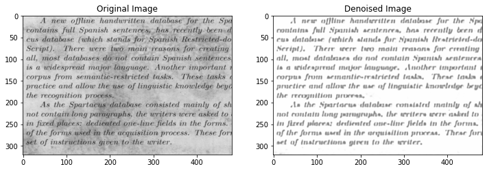
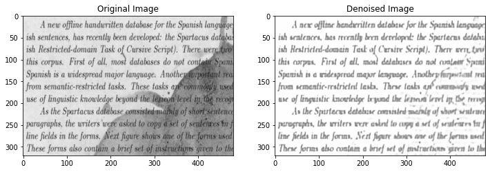
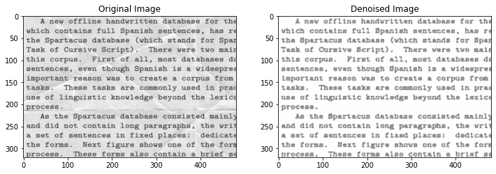
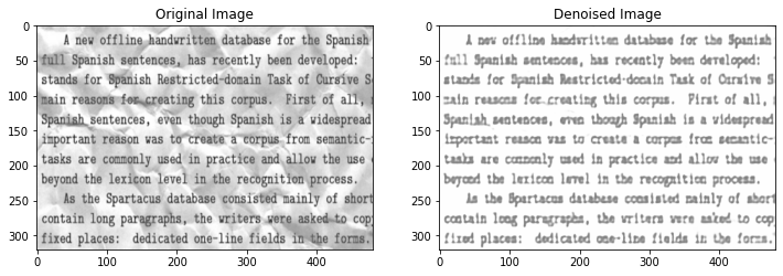
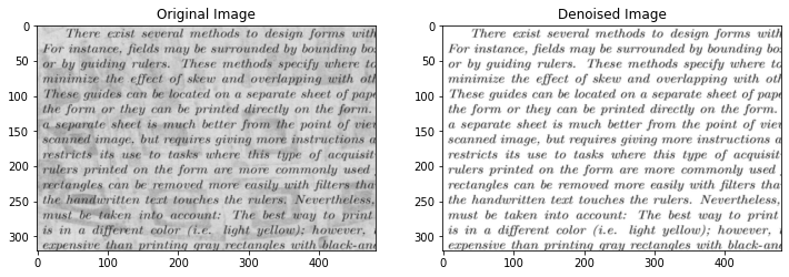
The train dataset contains two images for each entry, one of which is ‘clean’ and the other is ‘dirty’. As we will see, all the images are quite similar, rendering the same text with different fonts families and font sizes. There are only a few images: 144 in the training dataset and 72 in the test, but since they are all quite similar it will suffice.
data_dir = Path('./data')
train_dir = data_dir / 'train'
train_cleaned_dir = data_dir / 'train_cleaned'
test_dir = data_dir / 'test'

train_images = sorted(train_dir.glob('*.png'))
train_cleaned_images = sorted(train_cleaned_dir.glob('*.png'))
test_images = sorted(test_dir.glob('*.png'))

print('Number of Images in train:', len(train_images))
print('Number of Images in train_cleaned:', len(train_cleaned_images))
print('Number of Images in test:', len(test_images))
Number of Images in train: 144
Number of Images in train_cleaned: 144
Number of Images in test: 72
transform = transforms.Compose([
    transforms.Resize((320, 480)),
    transforms.ToTensor(),
    transforms.Normalize([0.5], [0.5]),
])

X = []
for image in train_images:
    pil_image = Image.open(image)
    pil_image = transform(pil_image)
    X.append(pil_image)

Y = []
for image in train_cleaned_images:
    pil_image = Image.open(image)
    pil_image = transform(pil_image)
    Y.append(pil_image)

test_images_transformed = []
for image in test_images:
    pil_image = Image.open(image)
    pil_image = transform(pil_image)
    test_images_transformed.append(pil_image)
def imshow(image, ax, title):
    if ax is None:
        fig, ax = plt.subplots()
    # PyTorch tensors assume the color channel is the first dimension
    # but matplotlib assumes is the third dimension
    image = image.transpose((1, 2, 0))

    # undo preprocessing
    mean = np.array([0.5, 0.5, 0.5])
    std = np.array([0.5, 0.5, 0.5])
    image = std * image + mean

    # image needs to be clipped between 0 and 1 or it looks like noise when displayed
    image = np.clip(image, 0, 1)

    ax.imshow(image)
    ax.grid(False)
    ax.set_title(title)
dataset = [(X[i], Y[i]) for i in range(len(X))]
random.shuffle(dataset)

split_size = 0.9
index = int(len(dataset)*split_size)

train_dataset = dataset[:index]
valid_dataset = dataset[index:]

train_loader = torch.utils.data.DataLoader(train_dataset, batch_size=32)
valid_loader = torch.utils.data.DataLoader(valid_dataset, batch_size=32)
images, targets = next(iter(train_loader))
images, targets = images.numpy(), targets.numpy()

def show_pair(i):
    plt.figure(figsize=(12, 14))
    ax = plt.subplot(1, 2, 1)
    imshow(images[i], ax, 'Original Image')
    ax = plt.subplot(1, 2, 2)
    imshow(targets[i], ax, 'Denoised Image')
for i in range(20):
    show_pair(i)
    plt.show()

The autoencoder itself is quite classical, with two layers of convolutional neural networks in the encoder and three such layers in the decoder. A max pool operator is used to reduce the image dimensions by half in each step, and an interpolator to extend the image dimensions in the decoder. The structure of the two is symmetric, as usual.
class DenoiserAutoencoder(nn.Module):

    def __init__(self):
        super().__init__();
        self.encoder1 = nn.Conv2d(1, 32, kernel_size=3, padding=1)
        self.encoder2 = nn.Conv2d(32, 64, kernel_size=3, padding=1)
        self.pool = nn.MaxPool2d(2, 2)
        self.decoder1 = nn.Conv2d(64, 64, kernel_size=3, padding=1)
        self.decoder2 = nn.Conv2d(64, 32, kernel_size=3, padding=1)
        self.decoder3 = nn.Conv2d(32, 1, kernel_size=3, padding=1)

    def forward(self, x):
        # encoding
        x = F.relu(self.encoder1(x))
        x = self.pool(x)
        x = F.relu(self.encoder2(x))
        x = self.pool(x)
        # decoding
        x = F.relu(self.decoder1(x))
        x = F.interpolate(x, scale_factor=2, mode='nearest')
        x = F.relu(self.decoder2(x))
        x = F.interpolate(x, scale_factor=2, mode='nearest')
        x = torch.sigmoid(self.decoder3(x))
        return x
model = DenoiserAutoencoder()
print(model)
DenoiserAutoencoder(
  (encoder1): Conv2d(1, 32, kernel_size=(3, 3), stride=(1, 1), padding=(1, 1))
  (encoder2): Conv2d(32, 64, kernel_size=(3, 3), stride=(1, 1), padding=(1, 1))
  (pool): MaxPool2d(kernel_size=2, stride=2, padding=0, dilation=1, ceil_mode=False)
  (decoder1): Conv2d(64, 64, kernel_size=(3, 3), stride=(1, 1), padding=(1, 1))
  (decoder2): Conv2d(64, 32, kernel_size=(3, 3), stride=(1, 1), padding=(1, 1))
  (decoder3): Conv2d(32, 1, kernel_size=(3, 3), stride=(1, 1), padding=(1, 1))
)
criterion = nn.MSELoss()
optimizer = torch.optim.Adam(model.parameters(), lr=0.001)

device = 'cpu'
if torch.cuda.is_available():
    device = 'cuda'
elif torch.has_mps:
    device = 'mps'
model = model.to(device)
print(f"Using device '{device}'")
Using device 'cpu'
def train(model, train_loader, valid_loader, num_epochs):

    for epoch in range(num_epochs):
        training_loss = 0.0
        for images, targets in train_loader:
            images, targets = images.to(device), targets.to(device)

            outputs = model(images)
            loss = criterion(outputs, targets)

            optimizer.zero_grad()
            loss.backward()
            optimizer.step()

            training_loss += loss.item()

        with torch.no_grad():
            valid_loss = 0
            for images, targets in valid_loader:
                images, targets = images.to(device), targets.to(device)

                outputs = model(images)
                loss = criterion(outputs, targets)

                valid_loss += loss.item()

        print(f'Epoch: {epoch + 1: 2d}/{num_epochs}    Training Loss: {training_loss/len(train_loader):.3f}    ' \
              f'Testing Loss: {valid_loss/len(valid_loader):.3f}')
train(model, train_loader, valid_loader, 50)
torch.save(model.state_dict(), './model.pt')
Epoch: 1/50    Training Loss: 0.273    Testing Loss: 0.228
Epoch: 2/50    Training Loss: 0.228    Testing Loss: 0.214
Epoch: 3/50    Training Loss: 0.208    Testing Loss: 0.195
Epoch: 4/50    Training Loss: 0.182    Testing Loss: 0.167
Epoch: 5/50    Training Loss: 0.159    Testing Loss: 0.150
Epoch: 6/50    Training Loss: 0.147    Testing Loss: 0.141
Epoch: 7/50    Training Loss: 0.138    Testing Loss: 0.134
Epoch: 8/50    Training Loss: 0.131    Testing Loss: 0.124
Epoch: 9/50    Training Loss: 0.124    Testing Loss: 0.121
Epoch: 10/50    Training Loss: 0.119    Testing Loss: 0.117
Epoch: 11/50    Training Loss: 0.116    Testing Loss: 0.113
Epoch: 12/50    Training Loss: 0.110    Testing Loss: 0.110
Epoch: 13/50    Training Loss: 0.107    Testing Loss: 0.106
Epoch: 14/50    Training Loss: 0.104    Testing Loss: 0.103
Epoch: 15/50    Training Loss: 0.101    Testing Loss: 0.100
Epoch: 16/50    Training Loss: 0.098    Testing Loss: 0.098
Epoch: 17/50    Training Loss: 0.095    Testing Loss: 0.096
Epoch: 18/50    Training Loss: 0.093    Testing Loss: 0.094
Epoch: 19/50    Training Loss: 0.091    Testing Loss: 0.092
Epoch: 20/50    Training Loss: 0.090    Testing Loss: 0.091
Epoch: 21/50    Training Loss: 0.088    Testing Loss: 0.089
Epoch: 22/50    Training Loss: 0.087    Testing Loss: 0.088
Epoch: 23/50    Training Loss: 0.085    Testing Loss: 0.086
Epoch: 24/50    Training Loss: 0.084    Testing Loss: 0.085
Epoch: 25/50    Training Loss: 0.082    Testing Loss: 0.083
Epoch: 26/50    Training Loss: 0.081    Testing Loss: 0.082
Epoch: 27/50    Training Loss: 0.079    Testing Loss: 0.081
Epoch: 28/50    Training Loss: 0.078    Testing Loss: 0.080
Epoch: 29/50    Training Loss: 0.077    Testing Loss: 0.078
Epoch: 30/50    Training Loss: 0.076    Testing Loss: 0.077
Epoch: 31/50    Training Loss: 0.075    Testing Loss: 0.076
Epoch: 32/50    Training Loss: 0.074    Testing Loss: 0.075
Epoch: 33/50    Training Loss: 0.073    Testing Loss: 0.075
Epoch: 34/50    Training Loss: 0.072    Testing Loss: 0.074
Epoch: 35/50    Training Loss: 0.072    Testing Loss: 0.074
Epoch: 36/50    Training Loss: 0.071    Testing Loss: 0.074
Epoch: 37/50    Training Loss: 0.071    Testing Loss: 0.075
Epoch: 38/50    Training Loss: 0.071    Testing Loss: 0.079
Epoch: 39/50    Training Loss: 0.072    Testing Loss: 0.083
Epoch: 40/50    Training Loss: 0.076    Testing Loss: 0.072
Epoch: 41/50    Training Loss: 0.074    Testing Loss: 0.073
Epoch: 42/50    Training Loss: 0.070    Testing Loss: 0.069
Epoch: 43/50    Training Loss: 0.068    Testing Loss: 0.070
Epoch: 44/50    Training Loss: 0.068    Testing Loss: 0.068
Epoch: 45/50    Training Loss: 0.067    Testing Loss: 0.067
Epoch: 46/50    Training Loss: 0.066    Testing Loss: 0.067
Epoch: 47/50    Training Loss: 0.065    Testing Loss: 0.066
Epoch: 48/50    Training Loss: 0.065    Testing Loss: 0.065
Epoch: 49/50    Training Loss: 0.064    Testing Loss: 0.065
Epoch: 50/50    Training Loss: 0.064    Testing Loss: 0.064
model.load_state_dict(torch.load('./model.pt'))
<All keys matched successfully>
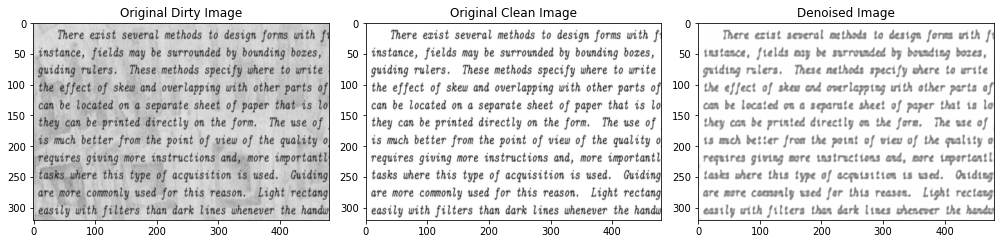
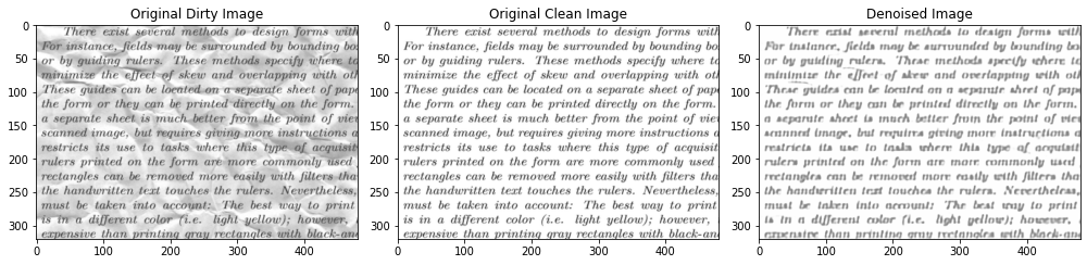
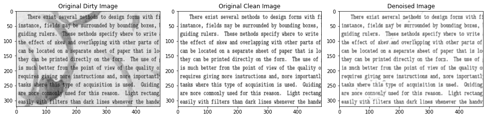
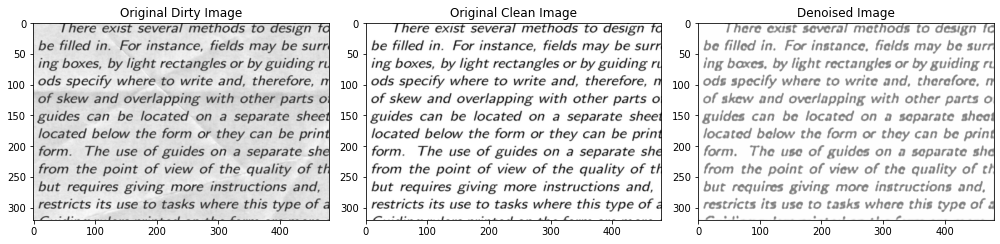
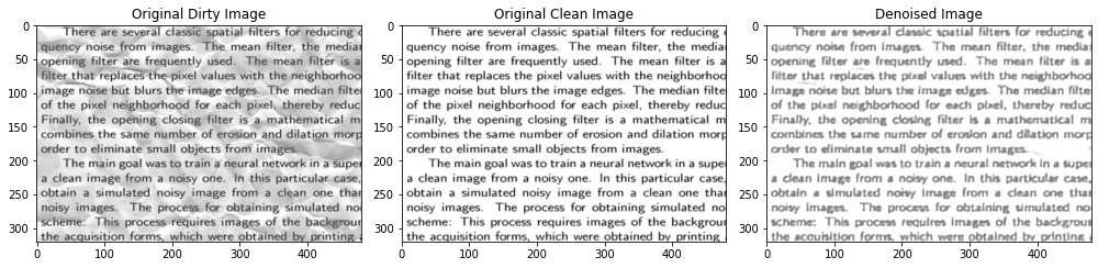
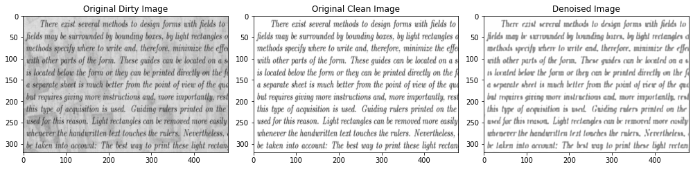
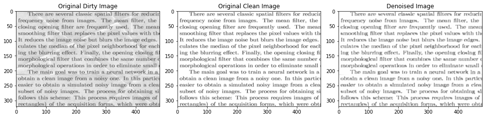
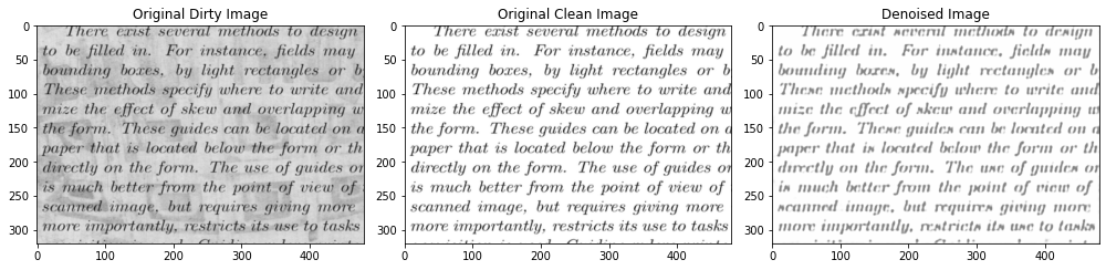
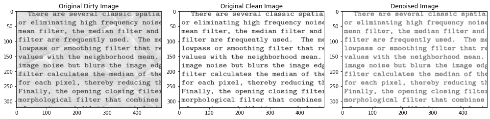
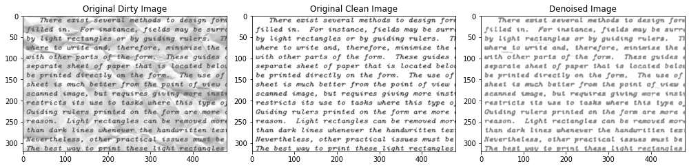
To analyze the performances, first we check the denoising on the training dataset, since we have the original clean image and the corresponding dirty one. Results are generally good, albeit sometimes the denoised image is too blurry.
def plot_triplet(n):
    fig, (ax0, ax1, ax2) = plt.subplots(figsize=(14, 8), ncols=3)
    image, image_clean = X[n], Y[n]
    image_pred = model(image.unsqueeze(0).to(device)).cpu().detach().numpy()
    imshow(image.numpy(), ax0, 'Original Dirty Image')
    imshow(image_clean.numpy(), ax1, 'Original Clean Image')
    imshow(image_pred.squeeze(0), ax2, 'Denoised Image')
    fig.tight_layout()
for n in random.sample(range(len(X)), 10):
    plot_triplet(n)
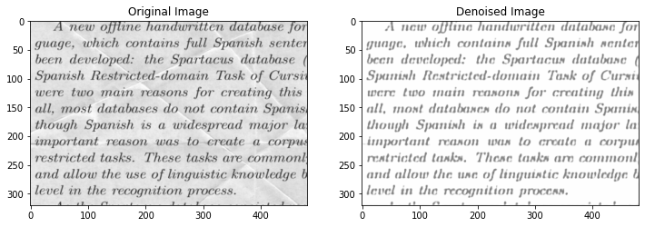
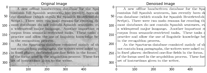
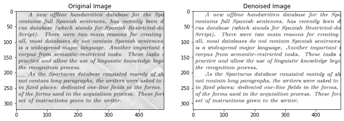
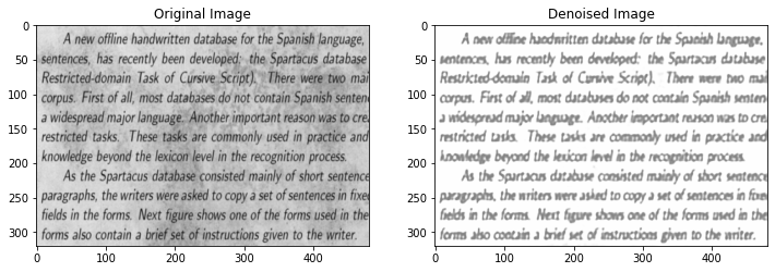
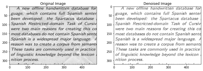
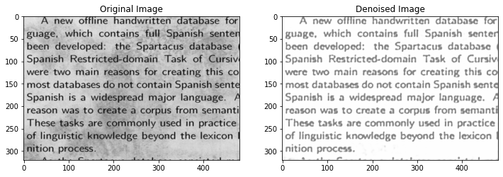
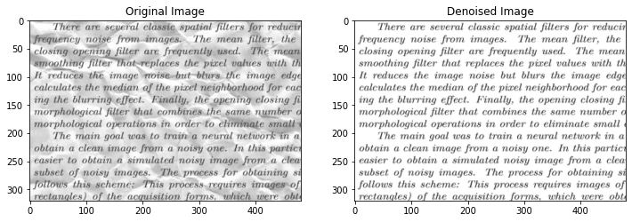
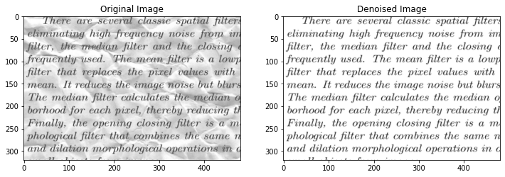
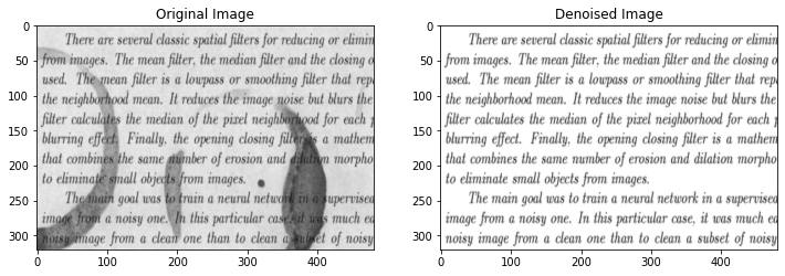
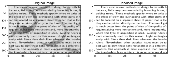
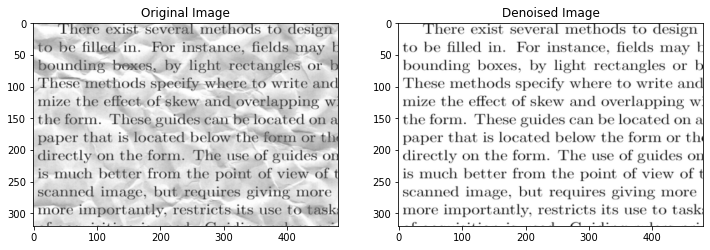
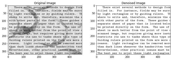
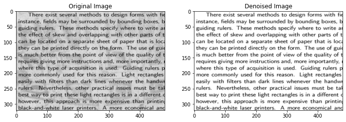
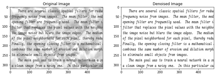
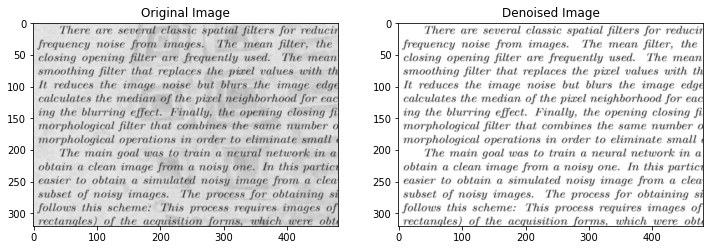
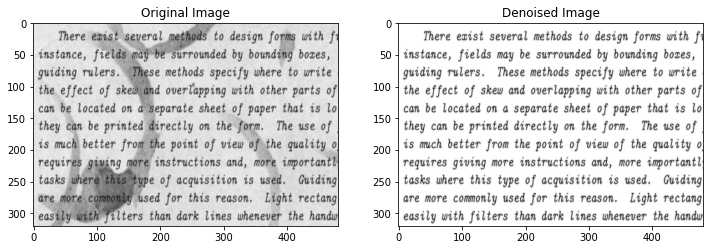
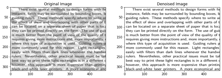
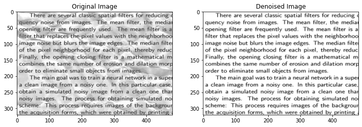
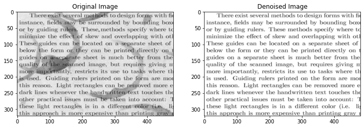
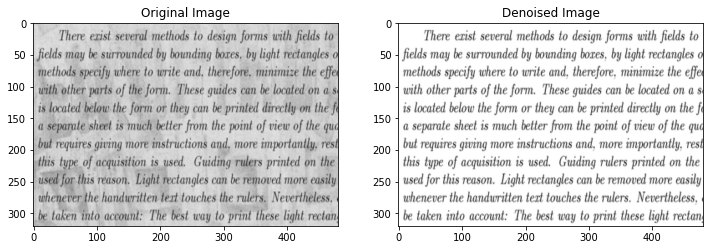
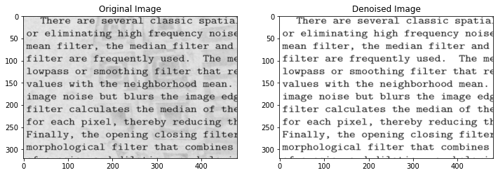
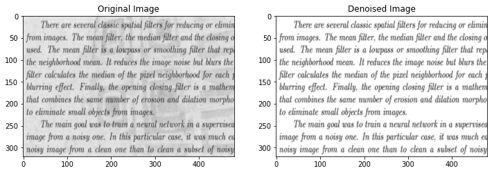
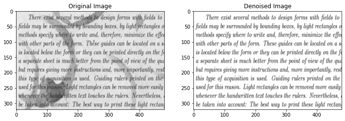
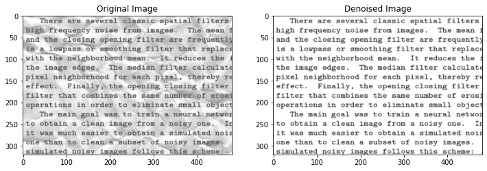
For the test dataset we only have the original (dirty image), so we plot that and the denoised one. When the noise is low-frequency compared with the text, results are excellent; instead when the text and the noise have similar frequencies, results are less good. Given the small size of the dataset, though, we can be quite satisfied by the performances of our autoencoder.
for n in random.sample(range(len(test_images)), 10):
    image = test_images_transformed[n]
    image = image.unsqueeze(0).to(device)
    output = model(image)

    image, output = image.detach().cpu().numpy(), output.detach().cpu().numpy()

    plt.figure(figsize=(12,14))
    ax = plt.subplot(1,2,1)
    imshow(image[0], ax, 'Original Image')

    ax = plt.subplot(1,2,2)
    imshow(output[0], ax, 'Denoised Image')

    plt.show()