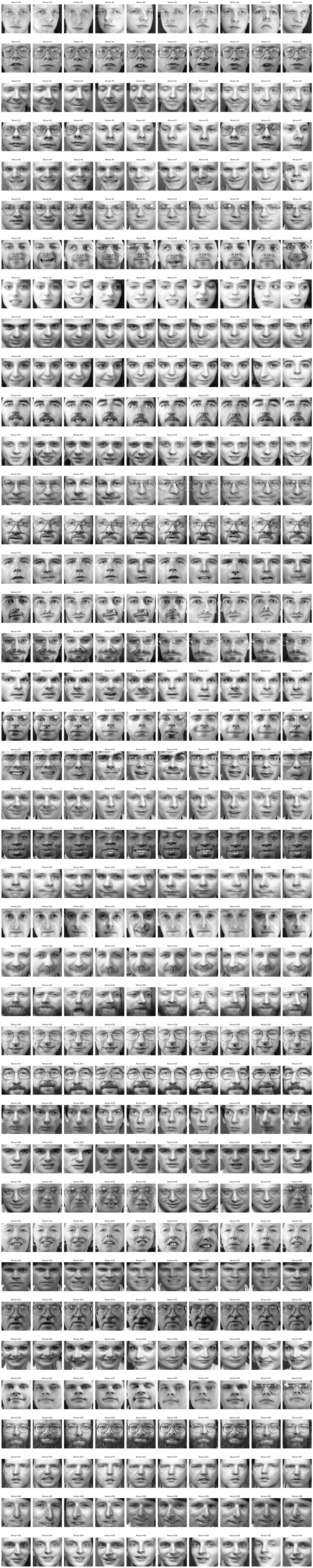
The Olivetti faces dataset is a small dataset that is part of the sklearn package. It contains 400 images, taken between April 1992 and April 1994 at AT&T Laboratories Cambridge. There are 40 different subjects, and for each subject there are ten different images, from a (slightly) different angle and with different conditions in lighting and facial expressions. All the images were taken against a dark homogeneous background with the subjects in an upright, frontal position (with tolerance for some side movement).
By today’s standards it is tiny; images are in black-and-white, with 256 levels of grey. The targets are numbers from 0 to 39, each of them corresponding to a different individual. In sklearn’s version, the images have a resolution of $64 \times 64$.
The goal of this article is to apply principal component analysis, or PCA, as a tool for dimensionality reduction.
from sklearn.datasets import fetch_olivetti_faces
from sklearn.decomposition import PCA
from sklearn.model_selection import train_test_split
import numpy as np
import pandas as pd
import seaborn as sns
import matplotlib.pyplot as plt
olivetti_faces = fetch_olivetti_faces()
num_samples, height, width = olivetti_faces.images.shape
X = olivetti_faces.data
num_features = X.shape[1]
y = olivetti_faces.target
num_classes = max(y) + 1

print(f"Number of samples: {num_samples}")
print(f"Images have height {height} and width {width}, total number of features: {num_features}")
print(f"Number of classes: {num_classes}")
Number of samples: 400
Images have height 64 and width 64, total number of features: 4096
Number of classes: 40
Since this is a very small dataset, we can plot it all. On each line, we render all the ten images for a given person. Those then images aren’t very different; they all represent the same part of the face (that is, they are well-centered already). Most of the subjects are male; 13 of them have glasses (of the shape then fashionable).
fig, axes = plt.subplots(figsize=(20, 100), ncols=10, nrows=40)
for i in range(40):
    current = X[y == i]
    for j in range(min(10, len(current))):
        axes[i, j].imshow(current[j].reshape((64, 64)), cmap=plt.cm.gray)
        axes[i, j].set_title(f'Person #{i}', fontsize=8)
    for j in range(10):
        axes[i, j].axis('off')
fig.tight_layout()
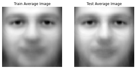
We will split randomly the dataset into two parts as customary, with the training set taking 75% of the data and the test set 25%.
X_train, X_test, y_train, y_test = train_test_split(X, y, test_size=0.25, random_state=42)
The average image is similar for the training and test sets, suggesting the split was balanced.
fig, (ax0, ax1) = plt.subplots(figsize=(8, 4), ncols=2)
ax0.imshow(np.mean(X_train, axis=0).reshape((64, 64)), cmap=plt.cm.gray)
ax0.axis('off')
ax0.set_title('Train Average Image')
ax1.imshow(np.mean(X_test, axis=0).reshape((64, 64)), cmap=plt.cm.gray)
ax1.axis('off')
ax1.set_title('Test Average Image');
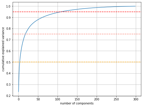
Computing PCA with sklearn is quite simple and, given the number of features and the size of the dataset, quite quick. Since the goal here is to understand what PCA does, we use 300 components, while in general people would use a smaller number.
num_components = 300
pca = PCA(n_components=num_components, whiten=False).fit(X_train)
The main idea of PCA is to take the first $n$ eigenvectors as they will explain most of the variance in the dataset. The plot below shows the explained variance (scaled such that the total variance is 1), while the horizontal lines report the values for 50%, 75% and 95% of the variance. A few eigenvalues easily explain 50% of the variance; we need between 20 and 30 for 75% of the variance, and about 100 for 95% of it.
plt.figure(figsize=(8, 6))
plt.plot(np.cumsum(pca.explained_variance_ratio_))
plt.xlabel('number of components')
plt.ylabel('cumulative explained variance')
plt.axhline(y=0.5, linestyle='dashed', color='orange')
plt.axhline(y=0.75, linestyle='dashed', color='salmon')
plt.axhline(y=0.95, linestyle='dashed', color='red')
plt.grid();
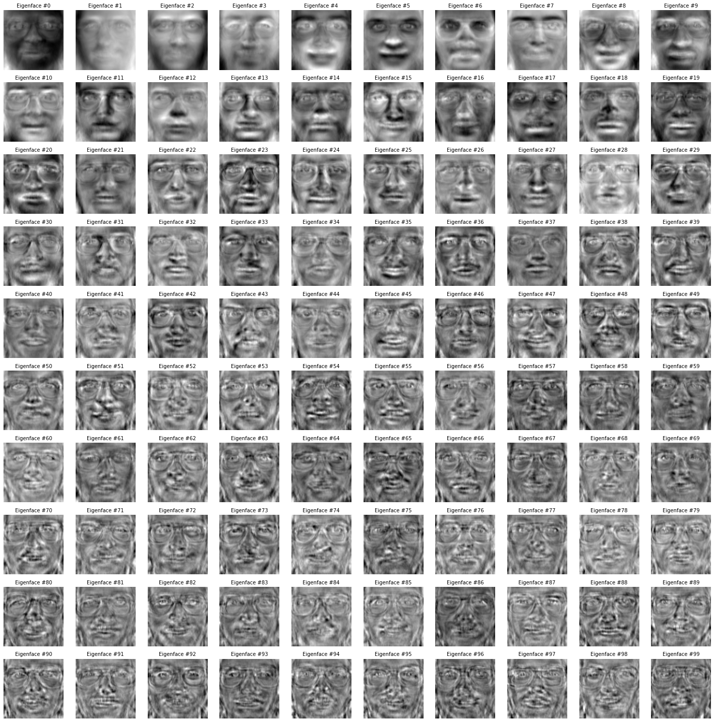
We can plot the so-called eigenfaces, that is the eigenvalues reshaped as an image. The first ones can be recognized as the main traits of a face, then changing slowly to what resembles more noise (or higher-frequency details).
eigenfaces = pca.components_.reshape((num_components, height, width))
fig, axes = plt.subplots(figsize=(20, 20), nrows=10, ncols=10)
axes = axes.flatten()
for i in range(100):
    axes[i].imshow(eigenfaces[i].reshape(64, 64), cmap=plt.cm.gray)
    axes[i].axis('off')
    axes[i].set_title(f'Eigenface #{i}', fontsize=10)
fig.tight_layout()
X_train_pca = pca.transform(X_train)
X_test_pca = pca.transform(X_test)
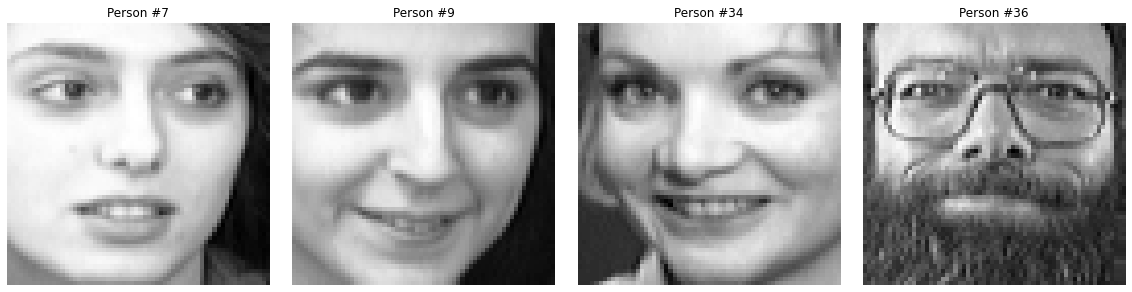
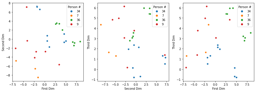
For a few images we can analyze their location on the coordinates given by the eigenvalues. We have selected four, three women and one man. Person #7 and person #9 are not very different; person #34 is a woman but different from #7 and #9, while #36 is quite different from the other three. Plotting the values on the first two dimensions of the eigenspace shows that the images for #7, #9 and #34 in separate clusters, with some points for #34 being close to that of #36; conclusions are less straightforward though on the scatter plot for the first and third eigenvalues and the second and third ones.
selected_ids = [7, 9, 34, 36]
fig, axes = plt.subplots(figsize=(16, 4), ncols=4)
for i, id in enumerate(selected_ids):
    axes[i].imshow(X_train[y_train == id][0].reshape(64, 64), cmap=plt.cm.gray)
    axes[i].axis('off')
    axes[i].set_title(f'Person #{id}')
fig.tight_layout()
subset = np.isin(y_train, selected_ids)
fix, (ax0, ax1, ax2) = plt.subplots(figsize=(15, 5), ncols=3)
df = pd.DataFrame({
    'First Dim': X_train_pca[subset, 0],
    'Second Dim': X_train_pca[subset, 1],
    'Third Dim': X_train_pca[subset, 2],
    'Person #': y_train[subset].astype(str),
})
sns.scatterplot(data=df, x='First Dim', y='Second Dim', hue='Person #', ax=ax0);
sns.scatterplot(data=df, x='Second Dim', y='Third Dim', hue='Person #', ax=ax1);
sns.scatterplot(data=df, x='First Dim', y='Third Dim', hue='Person #', ax=ax2);
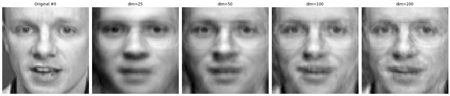
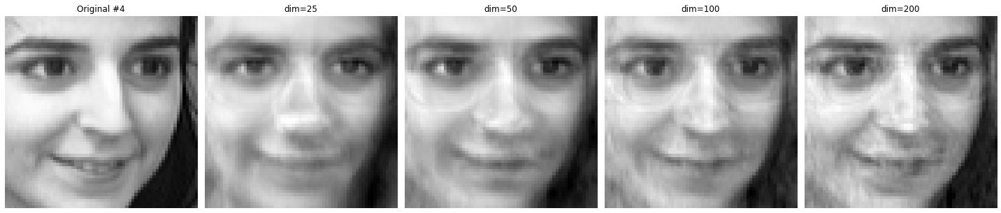
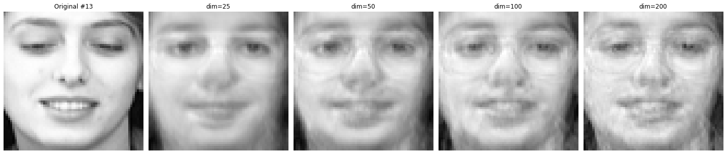
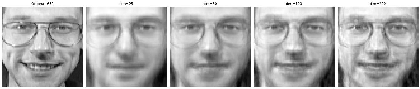
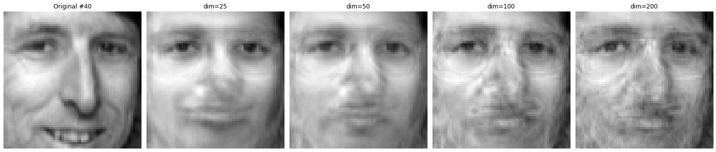
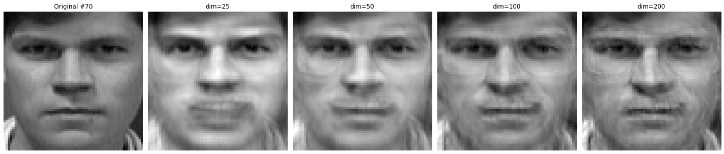
Another interesting analysis is to visualize the projection of the images into the subspace spanned by the first $n$ eigenvalues. The image on the left is the original one (from the test dataset); then we plot the projected image with the first 25, 50, 100 and 200 eigenfaces. Funnily, most projected images have some shapes around the eyes, even when the original one doesn’t.
def plot_reduced(i):
    fig, axes = plt.subplots(figsize=(20, 8), ncols=5)
    axes[0].imshow(X_test[i].reshape(64, 64), cmap=plt.cm.gray)
    axes[0].set_title(f'Original #{i}')
    axes[0].axis('off')
    for j, dim in enumerate([25, 50, 100, 200]):
        reduced = np.dot(X_test_pca[i, :dim], pca.components_[:dim, :]) + pca.mean_
        axes[j + 1].imshow(reduced.reshape(64, 64), cmap=plt.cm.gray)
        axes[j + 1].set_title(f'dim={dim}')
        axes[j + 1].axis('off')
    fig.tight_layout()
plot_reduced(0)
plot_reduced(4)
plot_reduced(13)
plot_reduced(32)
plot_reduced(40)
plot_reduced(70)
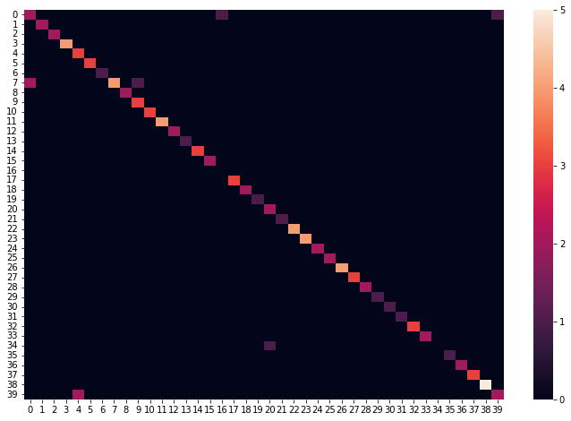
We conclude this analysis by training a classifier.
from sklearn.svm import SVC
from sklearn.metrics import classification_report
from sklearn.metrics import confusion_matrix
from sklearn import metrics
clf = SVC()
clf.fit(X_train_pca, y_train)
y_test_pred = clf.predict(X_test_pca)
print("accuracy score:{:.2f}".format(metrics.accuracy_score(y_test, y_test_pred)))
accuracy score:0.92
plt.figure(1, figsize=(12,8))
sns.heatmap(metrics.confusion_matrix(y_test, y_test_pred));
import warnings
warnings.filterwarnings("ignore")
print(metrics.classification_report(y_test, y_test_pred))
              precision    recall  f1-score   support

           0       0.50      0.50      0.50         4
           1       1.00      1.00      1.00         2
           2       1.00      1.00      1.00         2
           3       1.00      1.00      1.00         4
           4       0.60      1.00      0.75         3
           5       1.00      1.00      1.00         3
           6       1.00      1.00      1.00         1
           7       1.00      0.57      0.73         7
           8       1.00      1.00      1.00         2
           9       0.75      1.00      0.86         3
          10       1.00      1.00      1.00         3
          11       1.00      1.00      1.00         4
          12       1.00      1.00      1.00         2
          13       1.00      1.00      1.00         1
          14       1.00      1.00      1.00         3
          15       1.00      1.00      1.00         2
          16       0.00      0.00      0.00         0
          17       1.00      1.00      1.00         3
          18       1.00      1.00      1.00         2
          19       1.00      1.00      1.00         1
          20       0.67      1.00      0.80         2
          21       1.00      1.00      1.00         1
          22       1.00      1.00      1.00         4
          23       1.00      1.00      1.00         4
          24       1.00      1.00      1.00         2
          25       1.00      1.00      1.00         2
          26       1.00      1.00      1.00         4
          27       1.00      1.00      1.00         3
          28       1.00      1.00      1.00         2
          29       1.00      1.00      1.00         1
          30       1.00      1.00      1.00         1
          31       1.00      1.00      1.00         1
          32       1.00      1.00      1.00         3
          33       1.00      1.00      1.00         2
          34       0.00      0.00      0.00         1
          35       1.00      1.00      1.00         1
          36       1.00      1.00      1.00         2
          37       1.00      1.00      1.00         3
          38       1.00      1.00      1.00         5
          39       0.67      0.50      0.57         4

    accuracy                           0.92       100
   macro avg       0.90      0.91      0.91       100
weighted avg       0.93      0.92      0.92       100