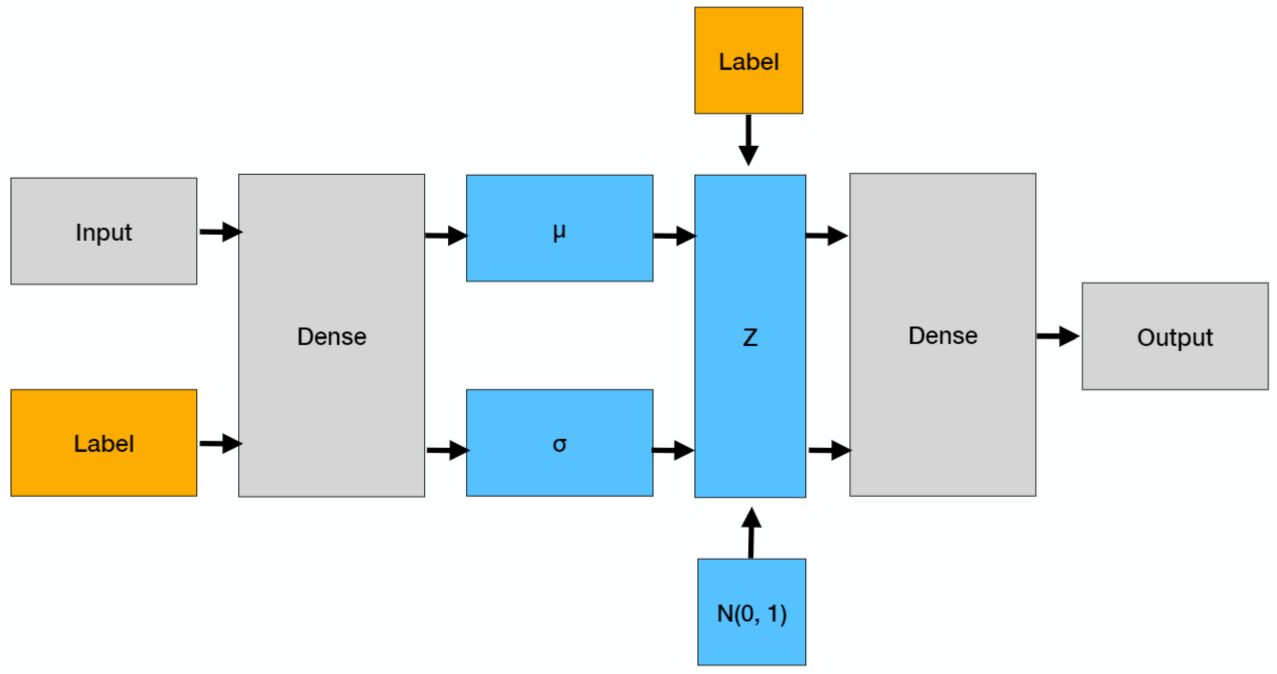
A conditional variational autoencoder is a generative method that is a simple extension of the variational autoencoders covered in the previous article. As we have seen, variational autoencoders can be very effective; however we have no control on the generated data, which can be problematic if we want to generate some specific data. A solution to this problem was proposed in a 2015 NIPS paper and consists in conditioning on the labels. This simple and elegant change means that both the encoder and the decoder take in input the label, as shown in the picture below, with the remainder equivalent to that of a variational autoencoder. We will use the Fashion MNIST dataset, provided by Zalando Research as a more challenging extension of the classical MNIST dataset. It contains 60,000 images for training and 10,000 images for testing; each image is associated to one of ten labels, where each label represents a fashion item. It is more complicated than MNIST, yet still reasonably easy for what we want to do here, which is to generate random objects belonging to each label.
import seaborn as sns
import torch; torch.manual_seed(0)
import torch.nn as nn
import torch.nn.functional as F
import torch.utils
import torch.distributions
import torchvision
import numpy as np
import matplotlib.pyplot as plt
Using a GPU reduces the computational time, so if one is available it’s better to take advantage of it.
device = 'cuda' if torch.cuda.is_available() else 'cpu'
print(f"Using device {device}")
Using device cuda
Our labels are categorical and we use a one-hot encoding.
def to_one_hot(index, n):

    assert torch.max(index).item() < n

    if index.dim() == 1:
        index = index.unsqueeze(1)
    onehot = torch.zeros(index.size(0), n).to(index.device)
    onehot.scatter_(1, index, 1)

    return onehot
This is the main part. The images, once flattened, have size 784. We use 256 hidden nodes in the first dense layer, which is connected to a dense layer to predict the means $\mu$ and the standard deviations $\sigma$. As $\sigma > 0$, we rather use $\log \sigma^2$, which is defined on the whole real axis.
class VariationalEncoder(nn.Module):

    def __init__(self, latent_dims, num_labels):
        super().__init__()
        self.linear = nn.Linear(784 + num_labels, 256)
        self.linear_mu = nn.Linear(256, latent_dims)
        self.linear_sigma = nn.Linear(256, latent_dims)
        self.num_labels = num_labels

        self.N = torch.distributions.Normal(0, 1)
        if device == 'cuda':
            self.N.loc = self.N.loc.cuda() # hack to get sampling on the GPU
            self.N.scale = self.N.scale.cuda()

    def forward(self, x, c):
        x = torch.flatten(x, start_dim=1)
        c = to_one_hot(c, self.num_labels)
        x = torch.cat((x, c), dim=1)
        x = F.relu(self.linear(x))
        mu =  self.linear_mu(x)
        sigma = torch.exp(self.linear_sigma(x))
        z = mu + sigma * self.N.sample(mu.shape)
        kl = (sigma**2 + mu**2 - torch.log(sigma) - 1/2).sum()
        return z, kl
The decoder is similar and takes in input the encodings as well as the digit c.
class Decoder(nn.Module):

    def __init__(self, latent_dims, num_labels):
        super(Decoder, self).__init__()
        self.linear1 = nn.Linear(latent_dims + num_labels, 256)
        self.linear2 = nn.Linear(256, 784)
        self.num_labels = num_labels

    def forward(self, z, c):
        c = to_one_hot(c, self.num_labels)
        z = torch.cat((z, c), dim=1)
        z = torch.sigmoid(self.linear1(z))
        z = torch.sigmoid(self.linear2(z))
        return z.reshape((-1, 1, 28, 28))
At this point creating the conditional autoencoder is trivial – just call one after the other, returning the prediction as well as the Kullback-Leibler distance.
class CVAE(nn.Module):

    def __init__(self, latent_dims, num_labels):
        super().__init__()
        self.encoder = VariationalEncoder(latent_dims, num_labels)
        self.decoder = Decoder(latent_dims, num_labels)
        self.num_labels = num_labels

    def forward(self, x, c):
        z, kl = self.encoder(x, c)
        return self.decoder(z, c), kl

    def compute_log_likelihood(self, X, X_hat, η):
        ξ = self.encoder.N.sample(X_hat.shape)
        X_sampled = X_hat + η * ξ
        return 0.5 * ((X - X_sampled)**2).sum() / η**2 + η.log()
We are now ready to load the data using Torch’s built-in functions. The batch size is 128.
data_set = torchvision.datasets.FashionMNIST('./data', transform=torchvision.transforms.ToTensor(),
                                             download=True)

data_loader = torch.utils.data.DataLoader(data_set, batch_size=128, shuffle=True)
From the Fashion MNIST website we get a description for each of the labels.
labels = {
    0: 'T-shirt/top',
    1: ' Trouser',
    2: ' Pullover',
    3: ' Dress',
    4: ' Coat',
    5: ' Sandal',
    6: ' Shirt',
    7: ' Sneaker',
    8: ' Bag',
    9: ' Ankle boot'
}
The train function is quite classical and similar to the one for variational autoencoders, with the difference that now the labels are used as well. We use 2 latent dimensions, which may be too little for this dataset, however it is the most convenient choice to visualize the results. The learning rate was set after a few tests and it is kept constant over all epochs.
def train(cvae, data_loader, epochs=20, lr=1e-4, η=0.1, print_every=10):
    η = torch.tensor(η)
    opt = torch.optim.Adam(cvae.parameters(), lr=lr)
    for epoch in range(epochs):
        total_loss = 0.0
        for x, y in data_loader:
            x, y = x.to(device), y.long().to(device)
            opt.zero_grad()
            x_hat, kl = cvae(x, y)
            log_loss = cvae.compute_log_likelihood(x, x_hat, η)
            loss = (log_loss + kl) / len(x)
            loss.backward()
            opt.step()
            total_loss += loss.item()
        if (epoch + 1) % print_every == 0:
            print(f"Epoch: {epoch + 1:3d}, loss: {total_loss:.4e}")
latent_dims = 2
cvae = CVAE(latent_dims, 10).to(device) # GPU
train(cvae, data_loader, epochs=1_000, lr=5e-3)
Epoch:  10, loss: 6.4921e+05
Epoch:  20, loss: 6.3496e+05
Epoch:  30, loss: 6.2825e+05
Epoch:  40, loss: 6.2401e+05
Epoch:  50, loss: 6.2119e+05
Epoch:  60, loss: 6.1866e+05
Epoch:  70, loss: 6.1669e+05
Epoch:  80, loss: 6.1601e+05
Epoch:  90, loss: 6.1398e+05
Epoch: 100, loss: 6.1367e+05
Epoch: 110, loss: 6.1244e+05
Epoch: 120, loss: 6.1198e+05
Epoch: 130, loss: 6.1082e+05
Epoch: 140, loss: 6.0986e+05
Epoch: 150, loss: 6.0948e+05
Epoch: 160, loss: 6.0856e+05
Epoch: 170, loss: 6.0907e+05
Epoch: 180, loss: 6.0775e+05
Epoch: 190, loss: 6.0778e+05
Epoch: 200, loss: 6.0665e+05
Epoch: 210, loss: 6.0611e+05
Epoch: 220, loss: 6.0603e+05
Epoch: 230, loss: 6.0593e+05
Epoch: 240, loss: 6.0541e+05
Epoch: 250, loss: 6.0528e+05
Epoch: 260, loss: 6.0502e+05
Epoch: 270, loss: 6.0443e+05
Epoch: 280, loss: 6.0471e+05
Epoch: 290, loss: 6.0409e+05
Epoch: 300, loss: 6.0435e+05
Epoch: 310, loss: 6.0290e+05
Epoch: 320, loss: 6.0316e+05
Epoch: 330, loss: 6.0311e+05
Epoch: 340, loss: 6.0247e+05
Epoch: 350, loss: 6.0257e+05
Epoch: 360, loss: 6.0271e+05
Epoch: 370, loss: 6.0162e+05
Epoch: 380, loss: 6.0264e+05
Epoch: 390, loss: 6.0226e+05
Epoch: 400, loss: 6.0231e+05
Epoch: 410, loss: 6.0187e+05
Epoch: 420, loss: 6.0170e+05
Epoch: 430, loss: 6.0127e+05
Epoch: 440, loss: 6.0130e+05
Epoch: 450, loss: 6.0106e+05
Epoch: 460, loss: 6.0075e+05
Epoch: 470, loss: 6.0111e+05
Epoch: 480, loss: 6.0163e+05
Epoch: 490, loss: 6.0129e+05
Epoch: 500, loss: 6.0107e+05
Epoch: 510, loss: 6.0087e+05
Epoch: 520, loss: 6.0019e+05
Epoch: 530, loss: 6.0036e+05
Epoch: 540, loss: 6.0005e+05
Epoch: 550, loss: 6.0059e+05
Epoch: 560, loss: 6.0040e+05
Epoch: 570, loss: 5.9997e+05
Epoch: 580, loss: 5.9922e+05
Epoch: 590, loss: 5.9961e+05
Epoch: 600, loss: 5.9978e+05
Epoch: 610, loss: 5.9968e+05
Epoch: 620, loss: 5.9926e+05
Epoch: 630, loss: 5.9873e+05
Epoch: 640, loss: 5.9929e+05
Epoch: 650, loss: 5.9894e+05
Epoch: 660, loss: 5.9842e+05
Epoch: 670, loss: 5.9874e+05
Epoch: 680, loss: 5.9838e+05
Epoch: 690, loss: 5.9874e+05
Epoch: 700, loss: 5.9852e+05
Epoch: 710, loss: 5.9917e+05
Epoch: 720, loss: 5.9836e+05
Epoch: 730, loss: 5.9944e+05
Epoch: 740, loss: 5.9813e+05
Epoch: 750, loss: 5.9815e+05
Epoch: 760, loss: 5.9783e+05
Epoch: 770, loss: 5.9775e+05
Epoch: 780, loss: 5.9850e+05
Epoch: 790, loss: 5.9846e+05
Epoch: 800, loss: 5.9813e+05
Epoch: 810, loss: 5.9730e+05
Epoch: 820, loss: 5.9774e+05
Epoch: 830, loss: 5.9809e+05
Epoch: 840, loss: 5.9734e+05
Epoch: 850, loss: 5.9794e+05
Epoch: 860, loss: 5.9779e+05
Epoch: 870, loss: 5.9819e+05
Epoch: 880, loss: 5.9745e+05
Epoch: 890, loss: 5.9771e+05
Epoch: 900, loss: 5.9742e+05
Epoch: 910, loss: 5.9811e+05
Epoch: 920, loss: 5.9710e+05
Epoch: 930, loss: 5.9669e+05
Epoch: 940, loss: 5.9729e+05
Epoch: 950, loss: 5.9675e+05
Epoch: 960, loss: 5.9713e+05
Epoch: 970, loss: 6.1050e+05
Epoch: 980, loss: 5.9678e+05
Epoch: 990, loss: 5.9672e+05
Epoch: 1000, loss: 5.9724e+05
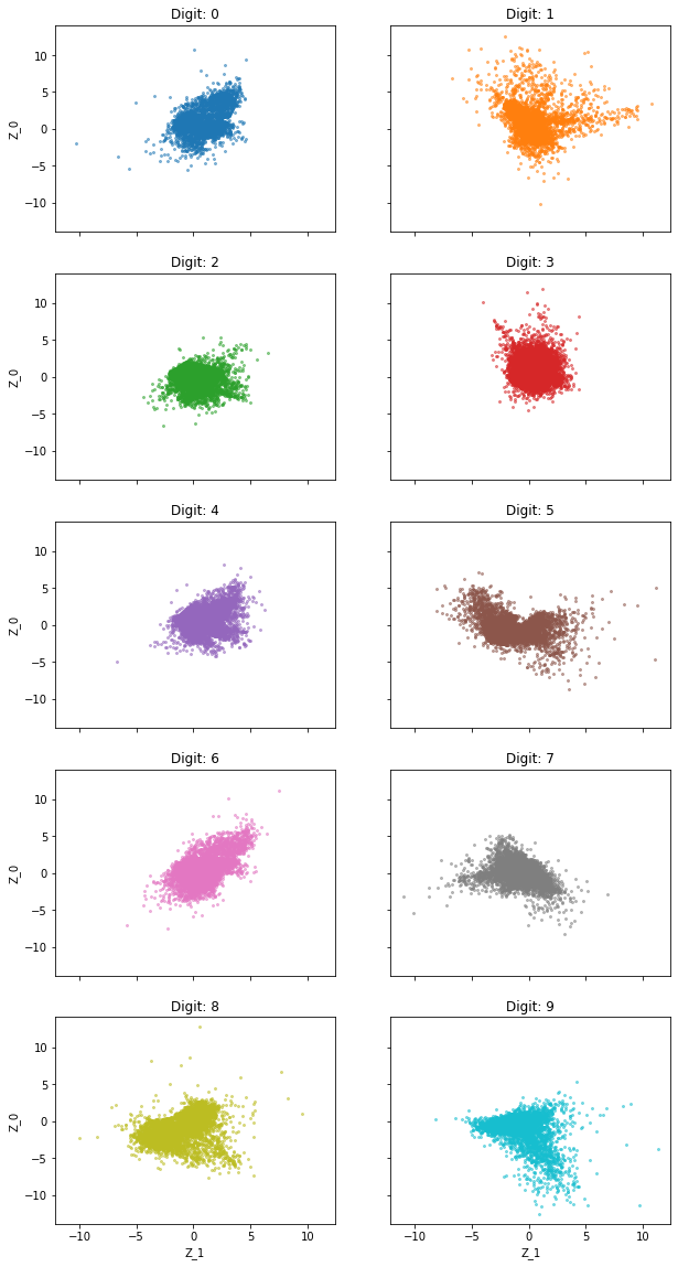
By plotting the encodings for each label, we notice that they are all reasonably well scattered around zero, even if not in the $(-3, 3)$ range expected from a standard random variable but in a slightly bigger one.
def plot_label(label, ax):
    colors = ['tab:blue', 'tab:orange', 'tab:green', 'tab:red', 'tab:purple',
              'tab:brown', 'tab:pink', 'tab:gray', 'tab:olive', 'tab:cyan']
    for x, y in data_loader:
        subset = y == label
        if sum(subset) == 0: continue
        x_label = x[subset].to(device)
        y_label = y[subset].to(device)
        z_label, _ = cvae.encoder(x_label, y_label)
        z_label = z_label.to('cpu').detach().numpy()
        ax.scatter(z_label[:, 0], z_label[:, 1], c=colors[label], s=4, alpha=0.5, cmap='tab10')
fig, axes = plt.subplots(figsize=(10, 20), nrows=5, ncols=2, sharex=True, sharey=True)
for row in range(5):
    for col in range(2):
        label = col + row * 2
        ax = axes[row, col]
        plot_label(label, ax)
        ax.set_title(f'Digit: {label}')
    axes[row, 0].set_ylabel('Z_0')
axes[4, 0].set_xlabel('Z_1')
axes[4, 1].set_xlabel('Z_1');
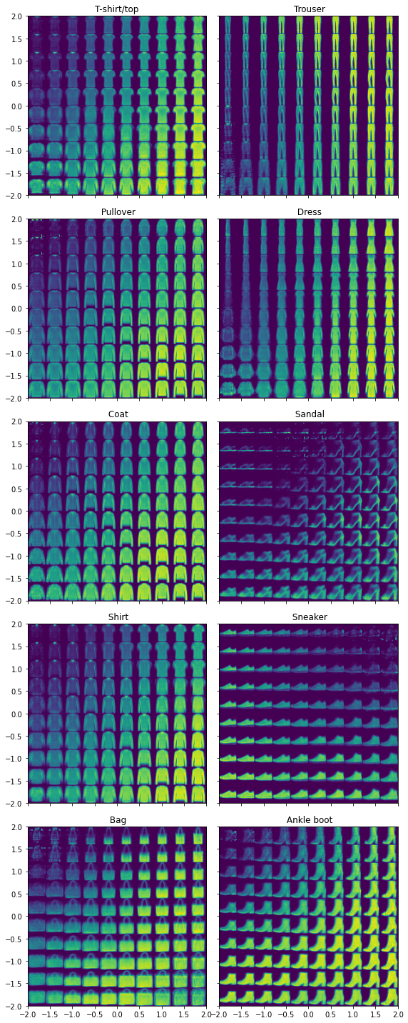
To look at the reconstructed digits, we go over the encoding space $(-2, 2) \times (-2, 2)$ for each digit. The results are quite good, with different styles for writing the numbers as we go from left to right and from top to bottom. Not all numbers are good (some of the four, eight and nine are badly written), yet overall we could easily generate digits that look realistic and have good quality.
def plot_reconstructed(cvae, digit, ax, r0=(-3, 3), r1=(-3, 3), n=20):
    w = 28
    img = np.zeros((n*w, n*w))
    for i, y in enumerate(np.linspace(*r1, n)):
        for j, x in enumerate(np.linspace(*r0, n)):
            z = torch.Tensor([[x, y]]).to(device)
            x_hat = cvae.decoder(z, torch.full_like(z, digit).long())
            x_hat = x_hat.reshape(28, 28).to('cpu').detach().numpy()
            img[(n-1-i)*w:(n-1-i+1)*w, j*w:(j+1)*w] = x_hat
    ax.imshow(img, extent=[*r0, *r1])
fig, axes = plt.subplots(figsize=(8, 20), nrows=5, ncols=2, sharex=True, sharey=True)
for row in range(5):
    for col in range(2):
        digit = col + row * 2
        ax = axes[row, col]
        plot_reconstructed(cvae, digit, ax, r0=(-2, 2), r1=(-2, 2), n=10)
        ax.set_title(labels[digit])
fig.tight_layout()