In this long article we explore the connection between stochastic differential equations (SDEs) and partial differential equations (PDEs). Our starting point is an SDE of type
\[\begin{align} dX(t) & = \mu(X(t), t) dt + \sigma(X(t), t) dW(t) \\ X(0) & = X_0, \end{align}\]for $t \in (t_0, T)$ and $W(t)$ a Wiener process. We want to compute
\[\mathbb{E}\left[ \Phi(X(T)) \right]\]for some function $\Phi(x)$. To solve numerically with Monte Carlo we define a time grid $0 = t_0 < t_1 < \ldots < t_m = T$, construct approximated paths
\[\hat X^{(\ell)}_i \approx X^{(\ell)}(t_i), \ell = 1, \ldots, N_{paths},\]and use the unbiased estimator
\[\mathbb{E}[\Phi(X(T))] \approx \frac{1}{N_{paths}} \sum_{\ell=1}^{N_{paths}} \Phi(\hat X_m^{(\ell)}).\]Another way for computing
\[\mathbb{E}[\Phi(X(T))]\]is to use partial differential equations. Let
\[u(x, t) = \mathbb{E}_{X(t)=x}[\Phi(X(T))].\]Then, $u(x, t)$ solves
\[\begin{cases} \displaystyle \frac{\partial{u(x, t)}}{\partial{t}} + \mu(x, t) \frac{\partial{u(x, t)}}{\partial{x}} + \frac{1}{2} \sigma(x, t)^2 \frac{\partial^2{u(x, t)}}{\partial{x^2}} = 0 & \text{ in } \mathbb{R} \times (0, T) \\ % u(x, T) = \Phi(x) & \text{ on } \mathbb{R}. \end{cases}\]This is known as the Feynman-Kac formula, which we will explore here.
To derive it, we apply Itô’s lemma to $u(X(t), t)$:
\[d[u(X(t), t)] = \left( \frac{\partial u}{\partial t} + \mu(x, t) \frac{\partial{u}}{\partial{x}} + \frac{1}{2} \sigma(x, t)^2 \frac{\partial^2{u}}{\partial{x^2}} \right) + \sigma(x, t) \frac{\partial u}{\partial x}dW(t),\]and integrate over time,
\[\begin{align} \displaystyle u(X(T), T) - u(X(t), t) = & \int_t^T \left( \frac{\partial u}{\partial t} + \mu(x, t') \frac{\partial{u}}{\partial{x}} + \frac{1}{2} \sigma(x, t')^2 \frac{\partial^2{u}}{\partial{x^2}} \right) dt'\\ & + \int_t^T \sigma(x, t') \frac{\partial u}{\partial x}dW(t'). \end{align}\]Taking expectations and using the final conditions yields $\mathbb{E}_{X(t)=x}[\Phi(X(T))] - u(x, t) = 0$, which is what we want to compute.
In general we are interested in some discounted payoff,
\[u(x, t) = \mathbb{E}_{X(t)=x} \left [e^{-\int_t^T r(X(s), s) ds }\Phi(X(T)) \right]\]for some known function $r(x, t)$, or if $r$ is not stochastic (and constant),
\[u(x, t) = e^{-r(T - t)} \mathbb{E}_{X(t)=x} \left [\Phi(X(T)) \right].\]Then $u(x, t)$ solves
\[\begin{cases} \displaystyle \frac{\partial{u(x, t)}}{\partial{t}} + \mu(x, t) \frac{\partial{u(x, t)}}{\partial{x}} + \frac{1}{2} \sigma(x, t)^2 \frac{\partial^2{u(x, t)}}{\partial{x^2}} -r(x, t) u = 0 & \text{ in } \mathbb{R} \times (0, T) \\ % u(x, T) = \Phi(x) & \text{ on } \mathbb{R}. \end{cases}\]An easy extension is for
\[u(x, t) = \mathbb{E}_{X(t) = x}\left[ \int_t^T \Psi(X(s), s) ds \right]\]for a specified function $\Psi$. Then $u(x, t)$ solves
\[\begin{cases} \displaystyle \frac{\partial{u(x, t)}}{\partial{t}} + \mu(x, t) \frac{\partial{u(x, t)}}{\partial{x}} + \frac{1}{2} \sigma(x, t)^2 \frac{\partial^2{u(x, t)}}{\partial{x^2}} + \Psi(x, t)= 0 & \text{ in } \mathbb{R} \times (0, T) \\ % u(x, T) = 0 & \text{ on } \mathbb{R}. \end{cases}\]This can be shown using as before Ito’s lemma:
\[\begin{align} d[u(x, t)] & = \underbrace{ \left( \frac{\partial{u}}{\partial{t}} + \mu(x, t) \frac{\partial{u}}{\partial{x}} + \frac{1}{2} \sigma(x, t)^2 \frac{\partial^2{u}}{\partial{x^2}} \right) }_{=-\Psi(X(t), t)} + \sigma(X(t), t) \frac{\partial u}{\partial x} dW(t) \\ & = -\Psi(X(t), t) dt + \sigma(X(t), t) \frac{\partial u}{\partial x} dW(t). \end{align}\]Integrating and taking expectations gives
\[\underbrace{u(X(T), T)}_{=0} - u(x, t) + \mathbb{E}_{X(t) = t}\left[ \int_t^T \Psi(X(s), s) ds \right] = 0.\]Another interesting case arises when integrating from $t$ to $\tau(x)$, the first time the process starting at $x=X(t)$ exits from some specified region $D \subset \mathbb{R}$. (If the process doesn’t exit from $D$, we set $\tau(x) = T$.) In this case the PDE must be solved in $D$ and not in $\mathbb{R}$. To evaluate
\[u(x, t) = \mathbb{E}_{X(t)=x} \left[ \Phi(X(\tau(x))) \right]\]we solve
\[\begin{cases} \displaystyle \frac{\partial{u(x, t)}}{\partial{t}} + \mu(x, t) \frac{\partial{u(x, t)}}{\partial{x}} + \frac{1}{2} \sigma(x, t)^2 \frac{\partial^2{u(x, t)}}{\partial{x^2}} = 0 & \text{ in } D \times (0, T) \\[1mm] % u(x, t) = \Phi(x, t) & \text{ on } \partial D \times (0, T). \\[1mm] % u(x, T) = \Phi(x, t) & \text{ on } D \end{cases}\]where $\Phi$ defines at the same time final and boundary conditions.
For example, what is the probability that our process exits the domain $D$ before time $T$? We can solve the equation
\[\begin{cases} \displaystyle \frac{\partial{u(x, t)}}{\partial{t}} + \mu(x, t) \frac{\partial{u(x, t)}}{\partial{x}} + \frac{1}{2} \sigma(x, t)^2 \frac{\partial^2{u(x, t)}}{\partial{x^2}} = 0 & \text{ in } D \times (0, T) \\[1mm] % u(x, t) = 1 & \text{ on } \partial D \times (0, T). \\[1mm] % u(x, T) = 0 & \text{ on } D. \end{cases}\]Changing the final and boundary conditions to
\[\begin{cases} u(x, t) = 0 & \text{ on } \partial D \times (0, T). \\[1mm] % u(x, T) = 1 & \text{ on } D \end{cases}\]yields the probability that the process does not exit $D$ before time $T$.
We now implement a simple solver of the above equations. First, we code a simple class to contain all the parameters for the SDE we want to solve, then we will use finite differences for the space discretization and the $\theta$-scheme for the time discretization of the Feynman-Kac equation.
from abc import ABC, abstractmethod
import matplotlib.pylab as plt
from matplotlib import cm
import numpy as np
import numpy.typing as npt
from numpy.polynomial.polynomial import polyfit, polyval
from scipy.linalg import solve_banded
All the quantities for such problem are contained in the SDE class. It contains the initial time $t_0$, usually set at 0.0, the final time $T$, the drift and diffusion coefficients $\mu(x, t)$ and $\sigma(x, t)$, as well as the function $\Phi$ that is used to compute the expectation. This simple class contains all that is needed to price with Monte Carlo.
class SDE(ABC):

    t_0: float

    T: float

    X_0: float

    def compute_μ(self, x, t):
        pass

    def compute_σ(self, x, t):
        pass

    def compute_Φ(self, x):
        pass
The corresponding backward PDE solution, instead, requires a few more classes. We start from the space and time domain, with time going from $t_0$ to $T$ and the domain from a value $x_{min}$ to an $x_{max}$.
class Domain:

    t_0: float

    T: float

    x_min: float

    x_max: float

    def __init__(self, t_0, T, x_min, x_max):
        assert t_0 < T
        assert x_min < x_max
        self.t_0 = t_0
        self.T = T
        self.x_min = x_min
        self.x_max = x_max
It is customary to solve PDE by moving forward in time, so we start with that: the InitialValueProblem class allows us to solve the equation
where $D = (x_{min}, x_{max})$. This is an equation that moves forward in time, so an additional step will be required to solve the Feynman-Kac equation, which we will do a bit later. The class InitialValuaProblem defines what is needed to solve the above equation: the coefficients $a(x, t)$, $b(x, t)$ and $c(x, t)$, the forcing term $f(x, t)$, the boundary conditions $g(x, t)$ and the initial condition $u_0(x)$. For simplicity we focus on Dirichlet boundary conditions and only note that other choices are possible.
The compute_u_exact() method is not strictly necessary but will be handy when we check the convergence of our schemes using the so-called method of manufactured solutions.
class InitialValueProblem(ABC):

    domain: Domain

    @abstractmethod
    def compute_a(self, x, t):
        "coefficient of the second-order derivative"
        pass

    @abstractmethod
    def compute_b(self, x, t):
        "coefficient of the first-order derivative"
        pass

    @abstractmethod
    def compute_c(self, x, t):
        "coefficient of the source term"
        pass

    @abstractmethod
    def compute_f(self, x, t):
        "force term"
        pass

    @abstractmethod
    def compute_g(self, x, t):
        "boundary conditions"
        pass

    @abstractmethod
    def compute_u_0(self, x):
        "initial condition"
        pass

    @abstractmethod
    def compute_u_exact(self, x, t):
        "the exact solution"
        pass
A concrete implementation of the abstract class is, for example, as below for constant coefficients.
class ConstantCoeffsInitialValueProblem(InitialValueProblem):

    def __init__(self, domain, a, b, c, exact_solution, f):
        self.domain = domain
        self.a = a
        self.b = b
        self.c = c
        self.exact_solution = exact_solution
        self.f = f

    def compute_a(self, x, t):
        return np.ones_like(x) * self.a

    def compute_b(self, x, t):
        return np.ones_like(x) * self.b

    def compute_c(self, x, t):
        return np.ones_like(x) * self.c

    def compute_f(self, x, t):
        return self.f(x, t)

    def compute_g(self, x, t):
        return self.exact_solution(x, t)

    def compute_u_0(self, x):
        return self.exact_solution(x, self.domain.t_0)

    def compute_u_exact(self, x, t):
        return self.exact_solution(x, t)
The discretization method is done using the method of lines, in which we first discretize in space and the in time.
The space discretization is handled by the SpaceDiscretizationMethod class to implement the discretization in space using finite differences. The class contains the member x_all that defines the spatial grid and two methods: assemble() is used to assemble the linear system matrix and impose_bc() will modify the linear system to impose the Dirichlet boundary conditions.
class SpaceDiscretizationMethod(ABC):

    problem: InitialValueProblem

    x_all: npt.NDArray

    @abstractmethod
    def assemble(self, t):
        pass

    @abstractmethod
    def impose_bc(self, t):
        pass
The parameters for the discretization are handled by a dictionary. A typical setup would be
params = dict(
    num_points=128,
    num_steps=64,
    time_integrator='Crank-Nicolson',
)
class SecondOrderFiniteDifferenceMethod(SpaceDiscretizationMethod):

    def __init__(self, problem: InitialValueProblem, params: dict):
        self.x_all = np.linspace(problem.domain.x_min, problem.domain.x_max, params['num_points'])
        self.problem = problem

    def assemble(self, t):
        num_points = len(self.x_all)
        A = np.zeros(num_points * 3)

        a = self.problem.compute_a(self.x_all, t)
        b = self.problem.compute_b(self.x_all, t)
        c = self.problem.compute_c(self.x_all, t)
        f = self.problem.compute_f(self.x_all, t)

        for i in range(1, num_points - 1):
            x_prev, x_i, x_next = self.x_all[i - 1], self.x_all[i], self.x_all[i + 1]
            h_prev, h_i = x_i - x_prev, x_next - x_i

            den = h_prev * h_i * (h_prev + h_i)

            D2_prev = 2 * h_i / den
            D2_i = -2 * (h_prev + h_i) / den
            D2_next = 2 * h_prev / den
            D1_prev = -1.0 / (h_prev + h_i)
            D1_next = 1.0 / (h_prev + h_i)

            A[i -1 + 2 * num_points] = a[i] * D2_prev + b[i] * D1_prev
            A[i + num_points] = a[i] * D2_i + c[i]
            A[i + 1] = a[i] * D2_next + b[i] * D1_next

        return A, f

    def impose_bc(self, t, A, f):
        num_points = len(self.x_all)

        A[1], A[num_points] = 0.0, 1.0
        A[-num_points - 1], A[-2] = 1.0, 0.0

        f[0] = self.problem.compute_g(self.x_all[0], t)
        f[-1] = self.problem.compute_g(self.x_all[-1], t)
For the time discretization, it is customary to use the \vartheta-method.
class ThetaMethod:

    def __init__(self, space_disc: SpaceDiscretizationMethod, params: dict):
        self.space_disc = space_disc
        self.t_all = np.linspace(space_disc.problem.domain.t_0, space_disc.problem.domain.T, params['num_steps'])
        if params['time_integrator'] == 'Crank-Nicolson':
            self.ϑ_all = np.ones_like(self.t_all) * 0.5
        elif params['time_integrator'] == 'Backward Euler':
            self.ϑ_all = np.ones_like(self.t_all)
        else:
            raise ValueError("time_integrator not recognized")

    @staticmethod
    def matmult(A, b):
        n = len(b)
        retval = A[n:2 * n] * b
        retval[:-1] += A[1:n] * b[1:]
        retval[1:] += A[2 * n:-1] * b[:-1]
        return retval

    def solve(self):
        n = len(self.space_disc.x_all)
        I = np.concatenate((np.zeros(n), np.ones(n), np.zeros(n)))

        u = self.space_disc.problem.compute_u_0(self.space_disc.x_all)
        solutions = [u]

        for k in range(len(self.t_all) - 1):
            t_k = self.t_all[k]
            t_k_plus_1 = self.t_all[k + 1]
            Δt = t_k_plus_1 - t_k

            ϑ = self.ϑ_all[k]

            A_k, f_k = self.space_disc.assemble(t_k)
            A_k_plus_1, f_k_plus_1 = self.space_disc.assemble(t_k_plus_1)

            Z = I - ϑ * Δt * A_k_plus_1
            b = self.matmult(I + (1 - ϑ) * Δt * A_k, u) + ϑ * Δt * f_k_plus_1 + (1 - ϑ) * Δt * f_k

            self.space_disc.impose_bc(t_k_plus_1, Z, b)

            u = solve_banded((1, 1), Z.reshape(3, -1), b)
            solutions.append(u)
        self.solutions = np.array(solutions)

    def get_solutions(self):
        return self.solutions

    def compute_max_error(self):
        max_error = 0.0
        u_T = self.solutions[-1]
        T = self.space_disc.problem.domain.T
        u_exact_T = self.space_disc.problem.compute_u_exact(self.space_disc.x_all, T)
        max_error = max(max_error, max(abs(u_T - u_exact_T)))
        return max_error
We run a simple test to verify the order of convergence. To do that, we first define the solution, then build the forcing term $f(x, t)$ such that the equation is satisfied.
ω = 4
α, β = 1, 10
a, b, c = 1.0, -2.0, 0.5
exact_solution = lambda x, t: np.sin(α * x + β * t)
der_t = lambda x, t: β * np.cos(α * x + β * t)
der_x = lambda x, t: α * np.cos(α * x + β * t)
der_xx = lambda x, t: -α**2 * np.sin(α * x + β * t)
f = lambda x, t: der_t(x, t) - a * der_xx(x, t) - b * der_x(x, t) - c * exact_solution(x, t)
domain = Domain(t_0=0, T=1.0, x_min=-np.pi, x_max=np.pi)
test = ConstantCoeffsInitialValueProblem(domain=domain, a=a, b=b, c=c, exact_solution=exact_solution, f=f)
hs = []
max_errors = []
base = 32
for η in [1, 2, 4, 8]:
    hs.append(1 / η)
    params = dict(num_points=16 * η, num_steps=16 * η, time_integrator='Crank-Nicolson')
    space_disc = SecondOrderFiniteDifferenceMethod(test, params)
    theta_method = ThetaMethod(space_disc, params)
    theta_method.solve()
    max_errors.append(theta_method.compute_max_error())
p = polyfit(np.log(hs), np.log(max_errors), 1)[1]
print(f"Convergence order: {p}")
Convergence order: 2.044773129350085
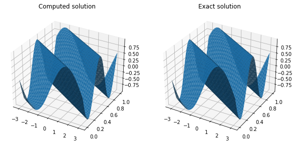
Plotting the solution shows good agreement between the exact and numerical solutions.
XX, YY = plt.meshgrid(space_disc.x_all, theta_method.t_all)
fig, (ax0, ax1) = plt.subplots(figsize=(10, 5), ncols=2,subplot_kw=dict(projection='3d'))
ax0.plot_surface(XX, YY, theta_method.solutions)
ax1.plot_surface(XX, YY, np.array([test.compute_u_exact(space_disc.x_all, t) for t in theta_method.t_all]))
ax0.set_title('Computed solution')
ax1.set_title('Exact solution');
We have tested our initial value problem solver: now we go back to the final value problem we need to solve. The move from backward to forward value problem is simple and involves a transformation from t to $\tau = T - t$, such that when $\tau=0$ we are at $t=T$, thus transforming the final conditions we need to impose for the Feynman-Kac into an initial condition. The coefficients $a(x, t)$, $b(x, t)$ and $c(x, t)$ are easily derived from $\mu(x, t)$ and $\sigma(x, t)$.
class FinalValueProblem(InitialValueProblem):

    def __init__(self, sde: SDE, x_min, u_min, x_max, u_max, f):
        self.sde = sde
        self.t_0 = sde.t_0
        self.T = sde.T
        self.domain = Domain(self.t_0, self.T, x_min, x_max)
        self.u_min = u_min
        self.u_max = u_max
        self.f = f

    def to_τ(self, t):
        return self.T - t

    def to_t(self, τ):
        return self.T - τ

    def compute_a(self, x, t):
        τ = self.to_τ(t)
        return 0.5 * self.sde.compute_σ(x, τ)**2

    def compute_b(self, x, t):
        τ = self.to_τ(t)
        return self.sde.compute_μ(x, τ)

    def compute_c(self, x, t):
        return np.zeros_like(x)

    def compute_f(self, x, t):
        return self.f(x, t)

    def compute_g(self, x, t):
        if x == self.domain.x_min:
            return self.u_min
        elif x == self.domain.x_max:
            return self.u_max
        else:
            raise Exception("9oundany condition not recognized")

    def compute_u_0(self, x):
        return self.sde.compute_Φ(x)

    def compute_u_exact(self, x, t):
        raise Exception("not implemented yet")
We will test a simple Wiener process, that is $\mu(x, t) = 0$ and $\sigma(x, t) = 1$, with $T=1$ and $\Phi(x) = Heaviside(x, 0)$.
class WienerProcess(SDE):

    def __init__(self, Φ):
        self.Φ = Φ

    t_0 = 0.0

    T = 1.0

    X_0 = 0.0

    def compute_μ(self, x, t) -> float:
        return np.zeros_like(x)

    def compute_σ(self, x, t) -> float:
        return np.ones_like(x)

    def compute_Φ(self, x):
        return self.Φ(x)
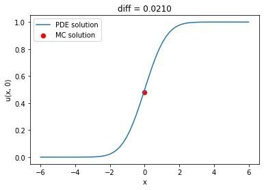
A basic Monte Carlo solver using the Euler-Maruyama method is easy to write; we will use it to check the PDE solution.
class MonteCarloMethod:

    def __init__(self, sde, num_paths, num_steps):
        self.t_all = np.linspace(0, sde.T, num_steps)
        X = sde.X_0 * np.ones(num_paths)
        X_all = [X]
        for i in range(num_steps - 1):
            t = self.t_all[i]
            Δt = self.t_all[i + 1] - t
            μ = sde.compute_μ(X, t)
            σ = sde.compute_σ(X, t)
            W = np.random.randn(num_paths)
            X = X + μ * Δt + σ * W * np.sqrt(Δt)
            X_all.append(X)
        self.X_all = np.array(X_all)
        self.Φ = sde.compute_Φ(X)

    def __call__(self):
        return self.Φ.mean()
f = lambda x, t: np.zeros_like(x)
wiener = WienerProcess(lambda x: np.where(x > 0, 1.0, 0.0))
problem = FinalValueProblem(wiener, -6.0, 0.0, 6.0, 1.0, f)
params = dict(num_points=64, num_steps=64, time_integrator='Crank-Nicolson')
space_disc = SecondOrderFiniteDifferenceMethod(problem, params)
theta_method = ThetaMethod(space_disc, params)
theta_method.solve()
mc_method = MonteCarloMethod(wiener, 1_000, 64)
mc_solution = mc_method()
pde_solution = np.interp(0.0, theta_method.space_disc.x_all, theta_method.solutions[-1])
plt.plot(theta_method.space_disc.x_all, theta_method.solutions[-1], label='PDE solution')
plt.scatter(0.0, mc_solution, s=40, color='red', label='MC solution')
plt.xlabel('x')
plt.ylabel('u(x, 0)')
plt.title(f'diff = {pde_solution - mc_solution:.4f}')
plt.legend();
We can also compute the probability of touching (or not touching) certain barriers. For example, what is the probability that a Wiender process starting at $X_0=0.0$ does not touch two barriers at $-1$ and $1$? Conversely, what is the probability that it does touch such barriers? To answer, we solve the Feymnan-Kac equation on $D=(-1, 1)$, imposing zero Dirichlet boundary conditions and unitary final condition for the no-touch case, and imposing unitary Dirichlet boundary conditions and zero final conditions for the non-touch case.
wiener = WienerProcess(lambda x: np.zeros_like(x))
problem = FinalValueProblem(wiener, -1.0, 1.0, 1.0, 1.0, f)
params = dict(num_points=64, num_steps=64, time_integrator='Crank-Nicolson')
space_disc = SecondOrderFiniteDifferenceMethod(problem, params)
theta_method = ThetaMethod(space_disc, params)
theta_method.solve()
solutions_touch = theta_method.solutions
wiener = wiener = WienerProcess(lambda x: np.ones_like(x))
problem = FinalValueProblem(wiener, -1.0, 0.0, 1.0, 0.0, f)
params = dict(num_points=64, num_steps=64, time_integrator='Crank-Nicolson')
space_disc = SecondOrderFiniteDifferenceMethod(problem, params)
theta_method = ThetaMethod(space_disc, params)
theta_method.solve()
solutions_no_touch = theta_method.solutions
XX, YY = plt.meshgrid(space_disc.x_all, theta_method.t_all)
fig, (ax0, ax1) = plt.subplots(figsize=(10, 5), ncols=2, subplot_kw=dict(projection='3d'),
                               sharex=True, sharey=True)
ax0.plot_surface(XX, YY, solutions_no_touch[::-1], cmap=cm.coolwarm, alpha=0.9)
ax0.scatter([0.0], [0.0], [np.interp(0.0, space_disc.x_all, solutions_no_touch[-1])], color='red', s=50)
ax0.set_title('No touch probability')
ax0.scatter(np.zeros(31), np.zeros(31), np.linspace(0., 1, 31), s=10, color='grey')
ax1.plot_surface(XX, YY, solutions_touch[::-1], cmap=cm.coolwarm, alpha=0.9)
ax1.scatter([0.0], [0.0], [np.interp(0.0, space_disc.x_all, solutions_touch[-1])], color='red', s=50)
ax1.scatter(np.zeros(31), np.zeros(31), np.linspace(0., 1, 31), s=10, color='grey')
ax1.set_title('Touch probability')
for ax in (ax0, ax1):
    ax.set_xlabel('x')
    ax.set_ylabel('t')
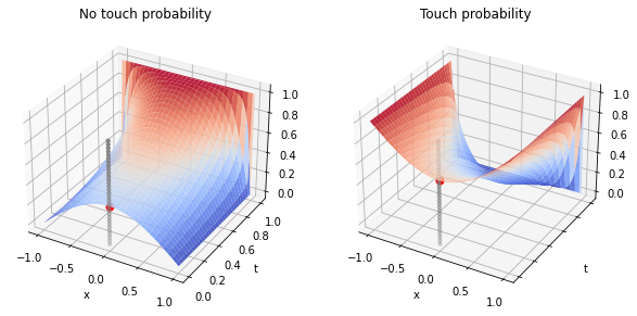
As the process can either touch or not touch the barriers, we expect the sum of the two probabilities to be one, and indeed it is:
np.interp(0.0, space_disc.x_all, solutions_no_touch[-1]) + np.interp(0.0, space_disc.x_all, solutions_touch[-1])
1.0000000000000167
This concludes our quick overview of the Feymna-Kac equation.