In this post we apply variational autoencoders to fonts, using this Kaggle dataset. The results below using the version in numpy format with handwritten data, but there is also another file without the handwritten data.
import torch
import torch.utils.data
from torch import nn, optim
from torch.nn import functional as F
from torchvision import datasets, transforms
from torchvision.utils import save_image

import numpy as np
import matplotlib.pyplot as plt
import matplotlib.gridspec as gridspec
import pandas as pd
import random
import seaborn as sns
data = np.load('./data/character_fonts (with handwritten data).npz')
images, labels = data['images'], data['labels']
print(f"Images shape: {', '.join(map(str, images.shape))}")
print(f"Labels shape: {', '.join(map(str, labels.shape))}")
Images shape: 762213, 28, 28
Labels shape: 762213
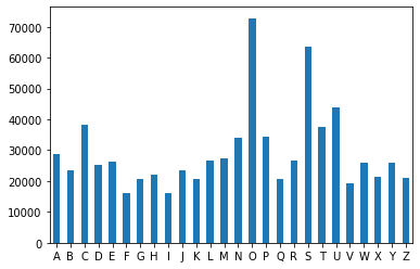
Letters do not all appear with the same frequency, as the histogram below shows. (They do for the non-handwritten dataset though.)
letters = [chr(i + ord('A')) for i in labels]
pd.Series(letters).value_counts().sort_index().plot.bar(x='Letter', y='# Samples', rot=0);
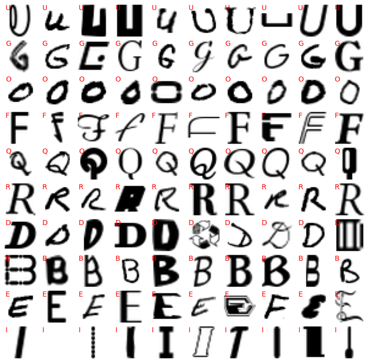
When displaying a few random entries, we see that the letters can have very different styles. Some entries look wrong or empty as well.
def show_images(nrows=10, ncols = 10):
    fig = plt.figure(figsize=(13, 13))
    ax = [plt.subplot(nrows, ncols, i + 1) for i in range(nrows * ncols)]
    temp = np.random.choice(np.arange(26), ncols, replace=False)
    count = -1
    l = []
    for i in temp:
        l.append(np.random.choice(np.argwhere(labels == i).ravel(),ncols, replace=False))
    for i, a in enumerate(ax):
        if i % ncols == 0:
            count += 1
        a.imshow(images[l[count][i % ncols]], cmap='gray_r')
        a.text(1, 5, letters[l[count][i % ncols]], color='red', fontsize=14)
        a.axis('off')
        a.set_aspect('equal')
    fig.subplots_adjust(wspace=0.0, hspace=0.05)
show_images()
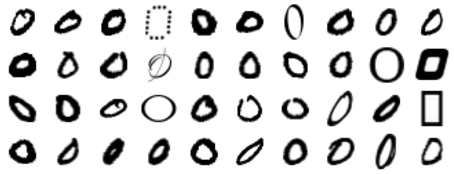
Let’s focus on the letter O, which should be simple enough to be described well by only two latent variables, and plot a few of them specifically.
chosen_letter = 'O'
subset = images[labels == ord(chosen_letter) - ord('A')]
print(f"Selected {len(subset)} image with the letter {chosen_letter}.")
Selected 72816 image with the letter O.
fig, axes = plt.subplots(nrows=4, ncols=10, figsize=(13, 5))
for ax in axes.flatten():
    ax.imshow(subset[np.random.randint(len(subset))], cmap='gray_r')
    ax.axis('off')
    ax.set_aspect('equal')
fig.subplots_adjust(wspace=0.0, hspace=0.05)
fig.tight_layout()
As customary, we divide the dataset into train and test, leaving 500 images for the testing and the rest for training.
dataset = torch.tensor(subset).unsqueeze(1) / 256
dataset_train, dataset_test = torch.utils.data.random_split(dataset, [len(dataset) - 500, 500])
dataloader_train = torch.utils.data.DataLoader(dataset_train, batch_size=64, shuffle=True)
dataloader_test = torch.utils.data.DataLoader(dataset_test, batch_size=64, shuffle=True)
The variational autoencoder isn’t that different from the ones on previous posts; this version is most often found on the web.
class VAE(nn.Module):

    def __init__(self, num_latent, num_hidden):
        super(VAE, self).__init__()

        self.fc1 = nn.Linear(28 * 28, num_hidden)
        self.fc_mean = nn.Linear(num_hidden, num_latent)
        self.fc_std_dev = nn.Linear(num_hidden, num_latent)
        self.fc3 = nn.Linear(num_latent, num_hidden)
        self.fc4 = nn.Linear(num_hidden, 28 * 28)

    def encode(self, x):
        h1 = F.relu(self.fc1(x))
        return self.fc_mean(h1), self.fc_std_dev(h1)

    def reparametrize(self, mu, logvar):
        std = torch.exp(0.5 * logvar)
        eps = torch.torch.rand_like(std)
        return mu + eps * std

    def decode(self, z):
        h3 = F.relu(self.fc3(z))
        return torch.sigmoid(self.fc4(h3))

    def forward(self, x):
        mu, logvar = self.encode(x.view(-1, 28 * 28))
        z = self.reparametrize(mu, logvar)
        return self.decode(z), mu, logvar
def loss_function(recon_x, x, mu, logvar):
    BCE = F.binary_cross_entropy(recon_x, x.view(-1, 28 * 28), reduction='sum')
    KLD = -0.5 * torch.sum(1 + logvar - mu.pow(2) - logvar.exp())
    return BCE + KLD
As said before, we only use two latent variables. Two is too little to really capture the dynamics of the fonts, however it gives us now nice visualizations of how the font changes along the two latent dimensions.
def evaluate(evaluate_data):
    model.eval()
    val_loss = 0.0
    with torch.no_grad():
        for data in evaluate_data:
            data = data.to(device)
            recon_batch, mu, logvar = model(data)
            val_loss += loss_function(recon_batch, data, mu, logvar)
    val_loss /= len(evaluate_data.dataset)
    return val_loss.item()
device = torch.device('cuda' if torch.cuda.is_available() else 'cpu')
model = VAE(num_latent=2, num_hidden=256).to(device)

optimizer = optim.Adam(model.parameters(), lr=1e-3)
model.train()
history = []
for epoch in range(1_000):
    train_loss = 0.0
    for data in dataloader_train:
        data = data.to(device)
        optimizer.zero_grad()
        recon_batch, mu, logvar = model(data)
        loss = loss_function(recon_batch, data, mu, logvar)
        train_loss += loss.item()
        loss.backward()
        optimizer.step()
    train_loss /= len(dataloader_train.dataset)
    test_loss = evaluate(dataloader_test)
    history.append((train_loss, test_loss))
history = np.array(history)
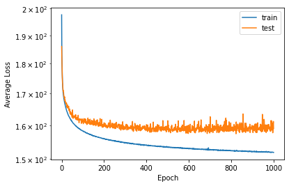
The convergence history shows a decreasing loss for both the training and the test set. One thousand iterations are too many, and we could have stopped after a few hundreds, as the average loss on the test set decreases by very little.
plt.semilogy(history[:, 0], label='train')
plt.semilogy(history[:, 1], label='test')
plt.xlabel('Epoch')
plt.ylabel('Average Loss')
plt.legend();
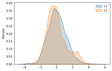
Another interesting graph is the distribution of the latent variables $(z_1, z_2)$. Ideally, they should be normal, that is the density plot should have the well-known bell shape. More or less this is what we get.
latent = []
for data in dataloader_train:
    data = data.to(device)
    mu, logvar = model.encode(data.view(-1, 28 * 28))
    z = model.reparametrize(mu, logvar)
    latent.append(z.detach().cpu())
latent = torch.cat(latent)

sns.kdeplot(latent[:, 0], shade=True, label='L1')
sns.kdeplot(latent[:, 1], shade=True, label='L2')
plt.legend()
<matplotlib.legend.Legend at 0x271b2ea6bc8>
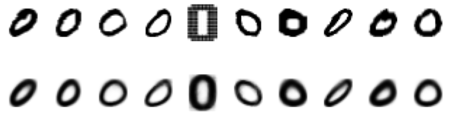
Let’s first see the quality of the reconstructed images – they are less sophisticated, as expected because there are only two parameters, but ok. Other letters, like F or Z, would not be reconstructed so well, but the O is simple enough.
fig, axes = plt.subplots(nrows=2, ncols=10, figsize=(13, 5))
for i in range(10):
    img = subset[random.randint(0, len(subset))]
    with torch.no_grad():
        img_recon = model(torch.tensor(img).to(device) / 256)
    axes[0, i].imshow(img, cmap='gray_r')
    axes[1, i].imshow(img_recon[0].view(28, 28).cpu(), cmap='gray_r')
    for ax in axes[:, i]:
        ax.axis('off')
        ax.set_aspect('equal')
fig.subplots_adjust(wspace=0.0, hspace=0.05)
fig.tight_layout()
And finally we can generate the images by using a grid of points for $(z_1, z_2)$. Since they are (or should be, at least) normally distributed, values between say $(-3, 3)$ or (-4, 4)$ would suit us well.
L = torch.linspace(-3, 3, 10)
with torch.no_grad():
    latent = []
    for i in L:
        for j in L:
            latent.append((i, j))
    latent = torch.tensor(latent).to(device)
    generated = model.decode(latent)
fig, axes = plt.subplots(nrows=10, ncols=10, figsize=(13, 13))
for ax, img in zip(axes.flatten(), generated):
    img = (img.view(28, 28).cpu() * 256).int()
    ax.imshow(img, cmap='gray_r')
    ax.axis('off')
    ax.set_aspect('equal')
fig.subplots_adjust(wspace=0.0, hspace=0.05)
fig.tight_layout()
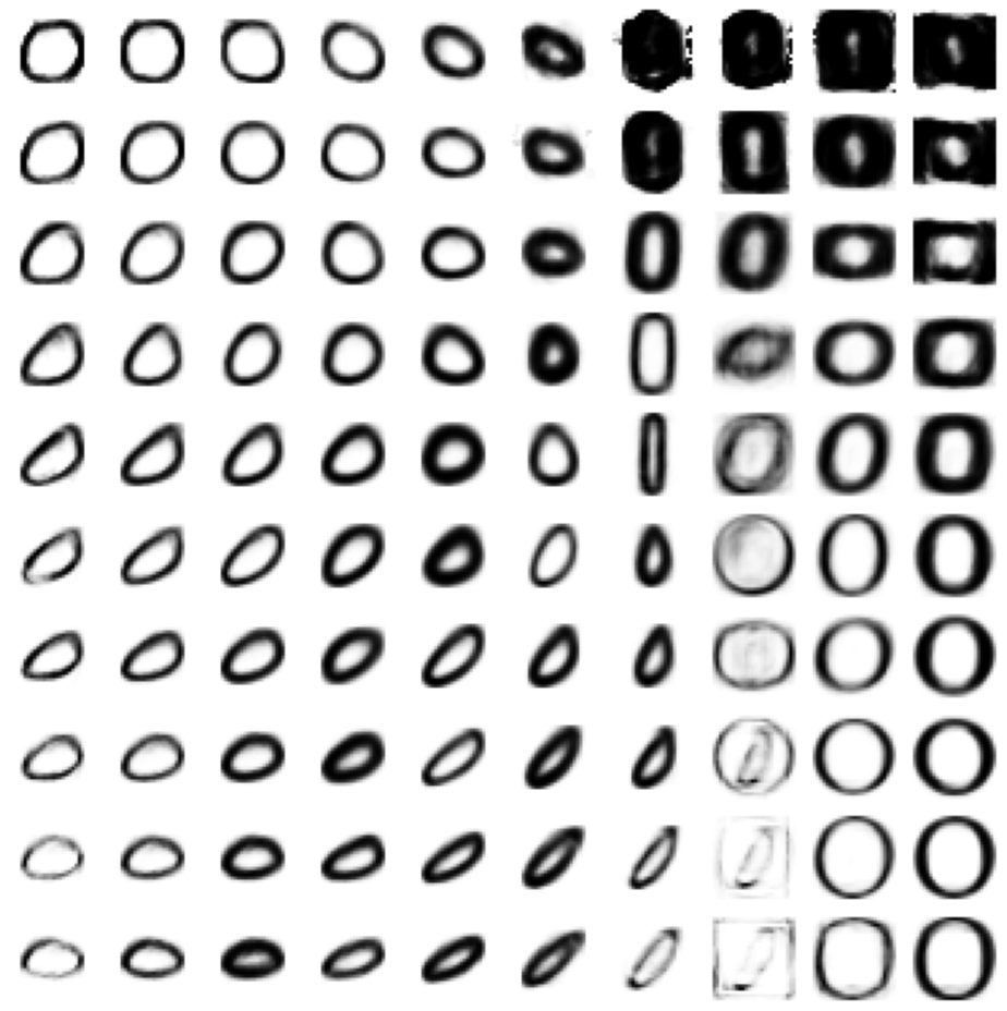
We can see the effect of the two parameters as we go over the rows and columns of the picture. On the top right the images aren’t very good, too dense, but all the others resemble the different styles for writing the letter O.