In this article we take a look at functional data analysis, a branch of statistics and data analysis that assumes that the observed data are generated by an underlying continuous stochastic process $X(t) \in L_2([a, b])$ with finite mean $\mu(t) = \mathbb{E}[X(t)]$ and variance, $\mathbb{E}[(X(t) - \mu(t))^2] < \infty$. By the Cauchy-Schwartz inequality, this implies that the covariance function $\mathbb{C}[s, t] = \mathbb{E}[(X(s) - \mu(s))(X(t) - \mu(t))]$ is finite as well, and the covariance function is exactly what we try to model and approximate.
Functional data is intrinsically infinite dimensional. This is both a challenge as well as an opportunity, because of the structure contained in the infinite dimensional space and the massive amount of information it contains. This is especially true if we assume that each realization has some smoothness requirements of the underlying (possibly stochastic) functional form, or mandate the existence of derivatives. In the following we also assume that this functional form is smooth — two adjancent data values are linked together and unlikely to be different. Often, this implies that our underlying process $X$ has one or more derivatives. (The observed data may not be smooth because of measurement errors or noise.)
The mathematical tool that underpins what we will do is the Kahrunen-Loève (KL) expansion, which is the decomposition of $X(t)$ into an infinite linear combination of orthogonal functions. Many such expansions exist; the importance of the KL expansion is that it yields the best such basis in the sense that it minimizes the total squared error.
Fourier series for non-stochastic processes are based on a fixed set of orthogonal functions (that is, sin and cos) and the coefficients of the series are fixed numbers; the KL expansions, instead, uses basis functions that depend on the process and the coefficients are random variables.
It can be defined as follows: $\forall t \in [a, b]$,
\[X(t) = \mu(t) + \sum_{k=1}^{\infty} Z_k \, \varphi_k(t),\]with $\varphi_k(t)$ continuous real-values fuctions and the $Z_k$ pairwise-uncorrelated (but not necessarily independent) random variables defined as
\[Z_k = \int_a^b (X(t) - \mu(t)) \, \varphi_k(t) dt\]where the ${ \varphi_k(t), k=1, \ldots, \infty }$ are the eigenfunction of the covariance operator. Often the terms $Z_k$ are called the scores. Also, and the coefficients ${ Z_k }$ have zeero mean and variance $\lambda_k$, where $\lambda_k$ is the eigenvalue corresponding to the $k$-th eigenfunction $\varphi_k(t)$, that is $\mathbb{E}[Z_K] = 0$ and $\mathbb{V}[Z_k] = \lambda_k$.
The series $\sum_{k=1}^{\infty} Z_k \, \varphi_k(t)$ converges in the mean squared error, uniformly in $t \in [a, b]$. Such feature has made this method and its generalizations very successful in applied disciplines. This is because it is a parsimonious description of functional data as it is the linear combination of the basis functions that explains the highest fraction of variance in the data with a given number of components. Its main attraction is the equivalence between $X(t)$ and the scores ${Z_1, Z_2, \ldots}$ such that any $X(t)$ can be expressed in terms of a countable sequence of uncorrelated scores, in decreasing order of importance (covariance-wise).
Karhunen-Loève Decomposition (KLD) is a widely used technique in functional data analysis (FDA) for representing and analyzing functional data. It is a dimensionality reduction method that transforms high-dimensional functional data into a lower-dimensional representation, retaining most of the variability in the data.
In an alternative form, we can define
\[Z_k^\star = \frac{Z_k}{\sqrt{\lambda_k}},\]obtaining
\[X(t) = \mu(t) + \sum_{k=1}^\infty \sqrt{\lambda_k} Z_k^\star \, \varphi_k(t),\]where $\mathbb{E}[Z_k^\star] = 0$ and $\mathbb{V}[Z_k^\star] = 1$. By using this form we can quickly evalute the variances,
\[\mathbb{V}[X(t)] = \mathbb[X(t)^2] - \mathbb{E}[X(t)]^2 = \sum_{k=1}^\infty \lambda_k \, \varphi_k(t)^2,\]and consequently the total variance of the process over $[a, b]$ is
\[\begin{align} \int_a^b \mathbb{V}[X(t)] dt & = \int_a^b \sum_{k=1}^\infty \lambda_k \, \varphi_k(t)^2 dt \\ % & = \sum_{k=1}^\infty \int_a^b \lambda_k \, \varphi_k(t)^2 dt \\ % & = \sum_{k=1}^\infty \lambda_k \int_a^b \varphi_k(t)^2 dt \\ % & = \sum_{k=1}^\infty \lambda_k, \end{align}\]since the convergence is the series is uniform by Mercer’s theorem. If the expansion is truncated after $N$ terms, we would explain
\[\sum_{k=1}^N \lambda_k / \sum_{k=1}^\infty \lambda_k\]of the total variance of the process.
In order to compute such an approximation numerically, the first step is the definition of a set of basis functions, that is the functions ${ \varphi_k(t), k=1, \ldots, \infty }$ above that are independent of each other and that can approximate arbitratrily well any functions by taking a weighted sum of a large number of such functions. Several choices are available:
- polynomials are easy to define and compute but tend to be oscillate and produce unstable results with higher orders;
- Fourier basis functions have excellent computational properties, especially if the observations are equally spaced, and are natural for describing periodic data, but they can be problematic if the data is not periodic;
- finite element basis functions can be very convenient for domain with complicated shapes; and
- splines combine the fast computations of polynomials with substantilly greater flexibility, often achieved with only a modest number of basis functions.
We will focus on splines. Splines are constructed by dividing the interval of validity into subintervals, with boundaries at points called “break points” or “knots” $\mathcal{K}$. In every subinterval the spline function is a polynomial of fixed degree $m$; generally the degree is the same in every subinterval. At each knot, neighboring polynomials are constraint to have a certain regularity, enforcing continuity up to a certain order of derivation. Often, splines are defined to be continuous up to the second derivative. We note that a multiple of a spline function is still a spline function, and since sums and differences of splines are also splines, any linear combination of splines remains a spline.
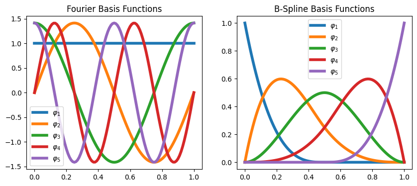
There are many ways to build our basis functions; here we consider B-splines, which are the most popular. B-splines have compact support: they are nonzero over no more than $m$ adjacent intervals, meaning that the matrix of the inner products of those functions will have a band structure, with only the elements up to $m-1$ from the diagional being nonzero. This is a substantial computational advantage when the number of basis functions increases.
Let’s first look at the construction of the basis functions using Python’s scikit-fda package. The locality of B-spline basis functions is apparent and constitues a strong incentive to use them for non-periodic data.
import matplotlib.pylab as plt
import numpy as np
import skfda
fig, (ax0, ax1) = plt.subplots(figsize=(10, 4), ncols=2)

basis = skfda.representation.basis.FourierBasis([0, 1], n_basis=5)
x = np.linspace(0, 1, 101)
y = basis(x).reshape(5, 101)
for i in range(5):
    ax0.plot(x, y[i, :], label=fr'$\varphi_{i + 1}$', linewidth=4)
ax0.legend()
ax0.set_title('Fourier Basis Functions')

basis = skfda.representation.basis.BSplineBasis(n_basis=5)
x = np.linspace(0, 1, 101)
y = basis(x).reshape(5, 101)
for i in range(5):
    ax1.plot(x, y[i, :], label=fr'$\varphi_{i + 1}$', linewidth=4)
ax1.legend()
ax1.set_title('B-Spline Basis Functions');
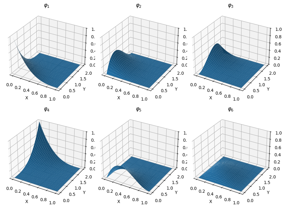
In multiple dimensions, the easiest approach is to combine single-dimension functions in a tensor basis. We plot a few of the resulting basis functions.
basis = skfda.representation.basis.TensorBasis([
    skfda.representation.basis.BSplineBasis(n_basis=4, domain_range=[0, 1]),
    skfda.representation.basis.BSplineBasis(n_basis=4, domain_range=[0, 2]),
])

XX, YY = plt.meshgrid(np.linspace(0, 1, 101), np.linspace(0, 2, 101))
ZZ = basis(np.vstack((XX.flatten(), YY.flatten())).T).reshape(16, 101 * 101)
fig = plt.figure(figsize=(9, 7))
axes = [fig.add_subplot(230 + k, projection='3d') for k in range(1, 7)]
for i, ax in enumerate(axes):
    ax.plot_surface(XX, YY, ZZ[i].reshape(101, 101))
    ax.set_xlabel('X')
    ax.set_ylabel('Y')
    ax.set_title(rf'$\varphi_{i + 1}$')
    ax.set_zlim(0, 1)
fig.tight_layout()
As an application, we consider the Kahrunen-Loève decomposition of a Wiener process $W(t)$ in $[0, 1]$, which can be computed and reads
\[W(t) = \frac{2 \sqrt{2}}{\pi} \sum_{k=1}^\infty \frac{Z_k^\star}{2k - 1} \sin \left( \frac{2(k -1) \pi}{2} t \right)\]where
\[\begin{align} Z_k & = \int_0^1 W(t)\sqrt{2} \sin\left( \frac{2(k-1)\pi}{2} t \right) dt \\ % \lambda_k & = \frac{4}{(2k - 1)^2 \pi^2} \\ % Z_k^\star & = \frac{Z_k}{\sqrt{\lambda_k}} \end{align}\]and the convergence in mean square is almost surely.
T = 1.0
num_steps = 100
sqrt_dt = np.sqrt(T / (num_steps + 1))
num_paths = 10000
X = np.zeros((1, num_paths))
X_all = [X]
for i in range(num_steps):
    W = np.random.randn(num_paths)
    X = X + sqrt_dt * W
    X_all.append(X)
X_all = np.concatenate(X_all).T
cov = np.cov(X_all.T)
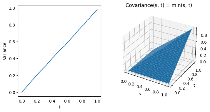
As expected, the variance grows linearly with $t$ and the covariance function is given by $\min(s, t)$.
fig = plt.figure(figsize=(8, 4))
ax0 = fig.add_subplot(121)
t_axis = np.linspace(0, T, num_steps + 1)
ax0.plot(t_axis, X_all.var(axis=0))
ax0.set_xlabel('t')
ax0.set_ylabel('Variance')

ax1 = fig.add_subplot(122, projection='3d')
XX, YY = plt.meshgrid(t_axis, t_axis)
ax1.plot_surface(XX, YY, cov)
ax1.set_xlabel('s')
ax1.set_ylabel('t')
ax1.set_title('Covariance(s, t) = min(s, t)');
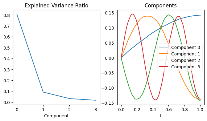
First we do the decomposition using principal component analysis. The result is not bad, however the scale isn’t correct.
from sklearn.decomposition import PCA
pca = PCA(n_components=4)
pca.fit(X_all)

fig, (ax0, ax1) = plt.subplots(figsize=(8, 4), ncols=2)
ax0.plot(pca.explained_variance_ratio_)
ax0.set_xlabel('Component')
ax0.set_title('Explained Variance Ratio')

for i in range(4):
    ax1.plot(t_axis, pca.components_[i], label=f'Component {i}')
ax1.legend()
ax1.set_xlabel('t')
ax1.set_title('Components');
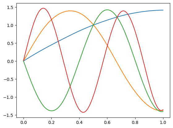
The KL decomposition using B-splines, instead, provides an accurate representation of the basis functions.
fd = skfda.FDataGrid(
    data_matrix=X_all,
    grid_points=t_axis,
)

basis = skfda.representation.basis.BSplineBasis(n_basis=10)
basis_fd = fd.to_basis(basis)

from skfda.preprocessing.dim_reduction import FPCA
fpca = FPCA(n_components=4)
fpca.fit(basis_fd)
fpca.components_.plot();
