Fractals

A fractal is a geometric shape containing detailed structure at arbitrarily small scales. What we will do in this article is to generate some of the nice pictures of fractals that we have all seen. The code is not difficult but there are a few tricks to take into account. Codewise it is convenient to use numba and its njit decorator to speed up the computations considerably, however the coding itself is quite simple. A bit trickier is to come up with a nice colormap that balances the warmth of the colors and the depth of the image – too few colors and the details are lost, too many colors and the image will look mostly of a single color with some hard-to-find spots here and there.

from functools import lru_cache
from numba import njit
from PIL import Image, ImageEnhance
import matplotlib.cm as cm
from matplotlib.colors import Normalize
from matplotlib import animation
import matplotlib.pylab as plt
import numpy as np

We will look at Julia and Mandelbrot sets, starting with the former. First the definition: a Julia set is computed by iteratively applying a function over a set of points in the complex plane. Mathematically, this looks like:

\[z_{n+1} = f(z_n)\]

where $c, z_n, z_{n+1} \in \mathbb{C}$ and $f(z_n) = z_n^2 + c$ is a nonlinear function. The function $f$ is applied recursively such that

\[z_{n + 1} = f(z_n) = f(f(z_{n-1})) = f(f(f \cdots f(z_0)))\]

where $z_0$ is a point on the complex plane. All the points for which $\lim_{n \rightarrow \infty} z_{n} = \infty$ are excluded from the set; what is left defined the Julia set. The zoom variable is used to zoom around the center of the image. What the compute_julia_set() function does is to compute, for each point in the image, at which iteration the recursive map goes to infinity. Small values means that we are in a highly diverging region; large values that we are in a region does either diverges very slowly or does not diverge at all.

@njit
def compute_julia_set(width, height, zoom, max_iters, c):
    image = np.zeros((width, height), dtype=np.int32)

    for x in range(width):
        for y in range(height):
            z_x = (x - width / 2) / (0.5 * zoom * width)
            z_y = (y - height / 2) / (0.5 * zoom * height)
            z = complex(z_x, z_y)
            for iter in range(max_iters):
                z = z**2 + c
                if z.real**2 + z.imag**2 >= 2:
                    break
            image[x, y] = iter
    return image

The get_rbg() function is responsible for converting the number of iterations before divergence (that is, the speed at which the point is going to infinity) to a RGB color. We use the lru_cache decorator to avoid repeated calls, as we only have a few colors anyway.

@lru_cache(maxsize=None)
def get_rbg(iter, max_iters):
    cmap = cm.Spectral
    norm = Normalize(vmin=0, vmax=max_iters)
    r, g, b, _ = cmap(norm(iter))
    return int(r * 255), int(g * 255), int(b * 255)

The array of iterations is converted into a proper image in create_image(), which takes in input the array of iterations as well as the maximum number of iterations we want to use in the colormap.

def create_image(image, max_iters):
    width, height = image.shape
    bitmap = Image.new("RGB", (width, height), "white")
    pix = bitmap.load()

    for x in range(width):
        for y in range(height):
            pix[x,y] = get_rbg(image[x, y], max_iters)
    return bitmap

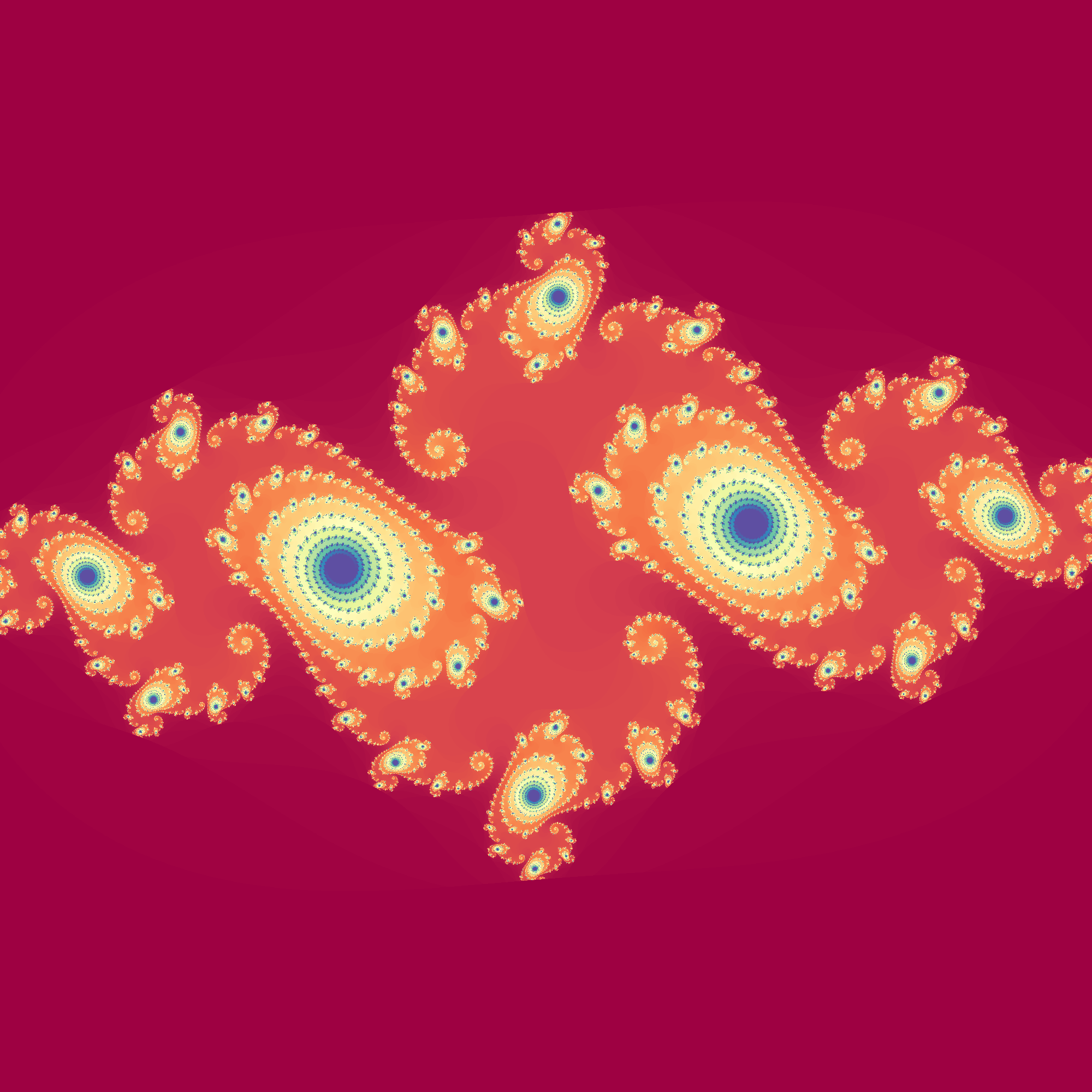
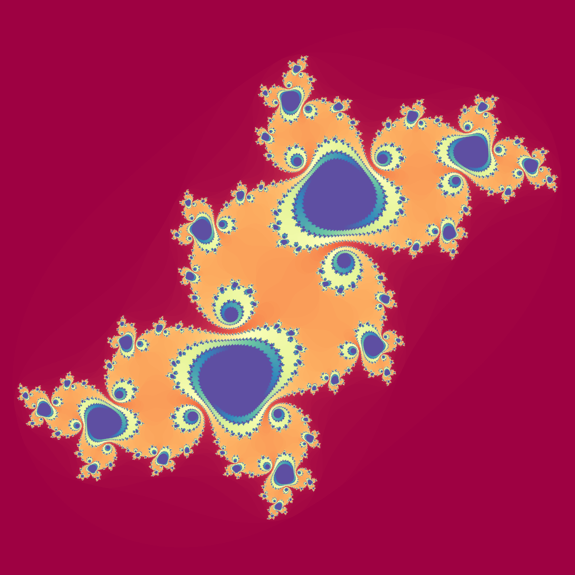
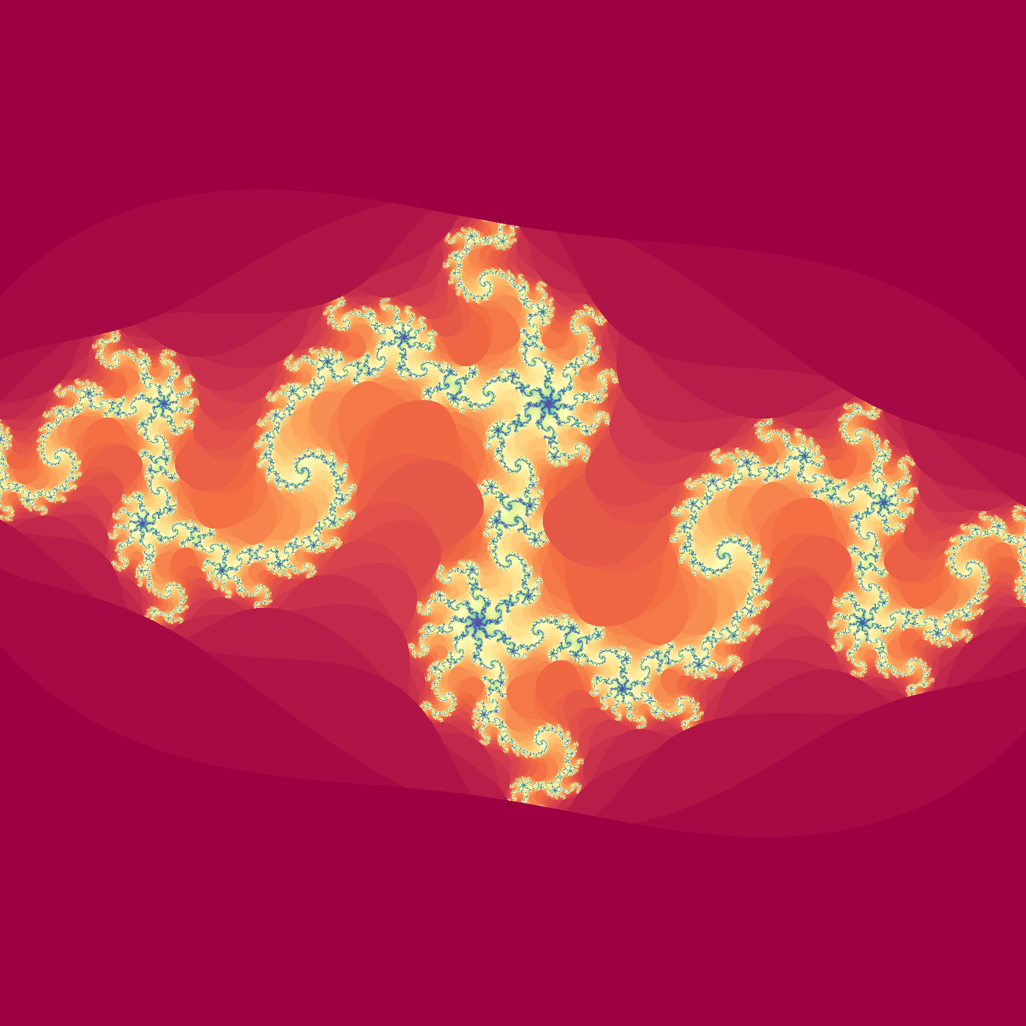
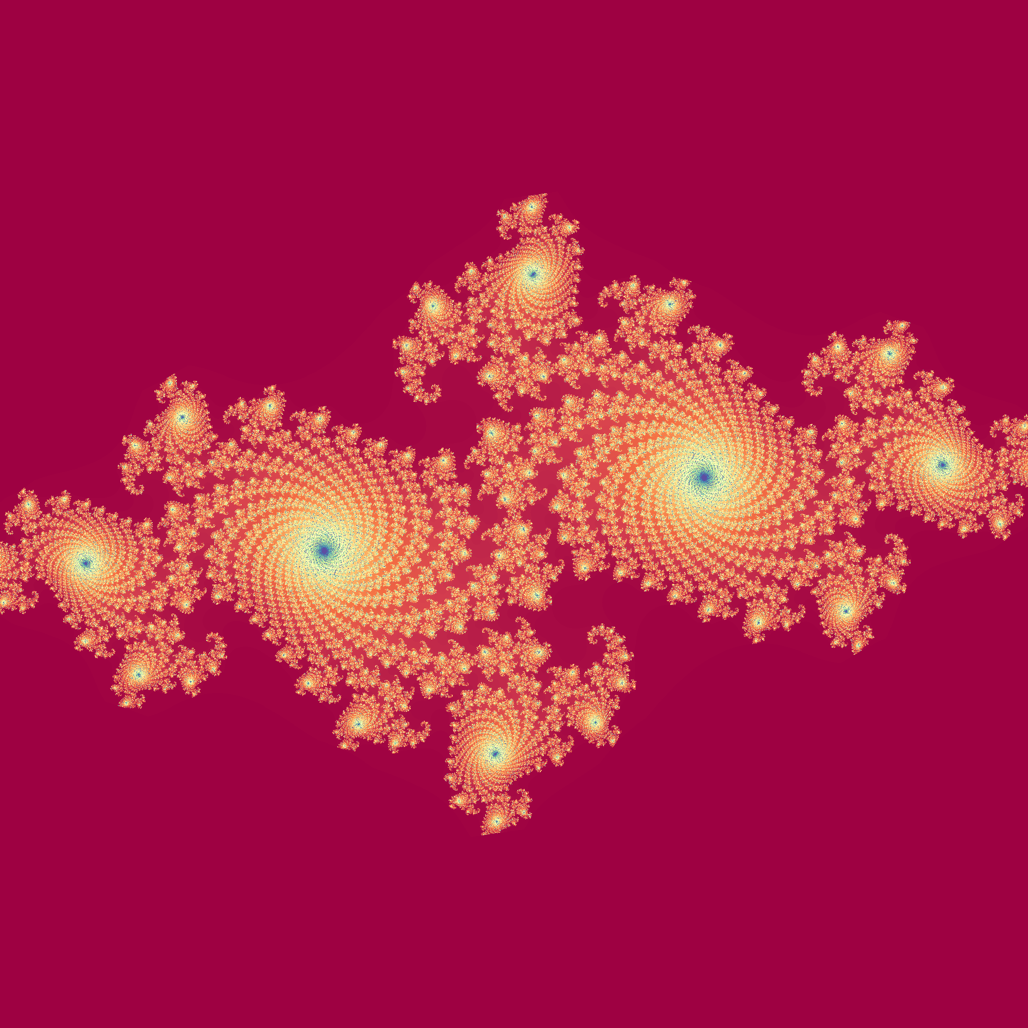
The Wikipedia web page on the Julia Set shows a few interesting ones and reports the values of $c$ that generates them, so let’s plot a few.

create_image(compute_julia_set(2000, 2000, 0.75, 256, -0.75 + 0.11j), 256)

create_image(compute_julia_set(2000, 2000, 0.75, 256, -0.1 + 0.651j), 256)

create_image(compute_julia_set(2000, 2000, 0.75, 256, -0.835 - 0.2321j), 64)

create_image(compute_julia_set(2000, 2000, 0.75, 1_024, -0.7269 + 0.1889j), 1_024)

A different but equally well-known fractal is Mandelbrot set, which consists of all of the values on the complex plane for which the corresponding orbit of 0 under $x^2 + c$ does not escape to infinity.

The code is just slightly different, but we approach from a different angle: we zoom around point $0.42611 + 0.198485 i$ and see the rich structure of the fractal, which reproduces itself over and over again as we go to smaller scales. The video generation takes a moment but it is well worth it.

@njit
def compute_mandelbrot_set(width, height, zoom, max_iters):
    image = np.zeros((width, height), dtype=np.int32)

    center = complex(0.42611, 0.198485)

    for x in range(width):
        for y in range(height):
            z = complex(0, 0)
            c_x = (x - width / 2) / (0.5 * zoom * width)
            c_y = (y - height / 2) / (0.5 * zoom * height)
            c = complex(c_x, c_y) + center
            for iter in range(max_iters):
                z = z**2 + c
                if z.real**2 + z.imag**2 >= 2:
                    break
            image[x, y] = iter
    return image

levels = [1.25**k for k in range(100)]
images = []
for zoom in levels:
    image = create_image(compute_mandelbrot_set(2000, 2000, zoom, 512), 512)
    enhancer = ImageEnhance.Brightness(image)
    enhancer.enhance(2)
    images.append(np.array(image))

video = np.array(images[:]) 

fig = plt.figure(figsize=(8, 8))
im = plt.imshow(video[0,:,:,:])
plt.axis('off')
plt.close() # this is required to not display the generated image

def init():
    im.set_data(video[0,:,:,:])

def animate(i):
    im.set_data(video[i,:,:,:])
    return im

anim = animation.FuncAnimation(fig, animate, init_func=init, frames=video.shape[0], interval=150)
anim.save('mandelbrot-zoom.gif', writer='pillow')

This concludes our short excursion on fractals. The video was the fun part and it will be nice to extend it to continue zooming even more.