In this article we explore fractional calculus, a branch of mathematics that extends the classical concept differentiation, which is defined for integers only, to a non-integer number $\alpha$. By notation, we use
\[D^\alpha f(x) = \frac{d^\alpha}{dx^\alpha} f(x).\]Using this notation, $D^0 f(x) = f(x)$ is the identity operator, $D^1 f(x)$ the first derivative, $D^2 f(x)$ the second derivative, and so on. We will also use $D^{-1} f(x)$ to define the integration of $f(x)$ over an unspecified interval. We expect
\[D^\alpha(\lambda f(x)) = \lambda D^\alpha f(x), \quad \lambda \in \mathbb{R}\]and
\[D^\alpha(f(x) + g(x)) = D^\alpha f(x) + D^\alpha g(x),\]from which it easily follows $D^\alpha 0$ = 0 and $D^\alpha 1 = 0$. Another property is
\[D^\alpha \left[ D^\beta f(x) \right] = D^{\alpha + \beta} f(x).\]Finally, we also expect any definition of $D^\alpha$ to recover the classical definition when $\alpha \in \mathbb{N}$. Our goal is to define such an operator.
We will start with an intuitive argument that works well with polynomials. When $f(x) = x^m$, we have
\[D^\alpha x^m = \frac{m!}{(m - \alpha)!}x^{m - \alpha},\]with $m \ge \alpha$. Using Euler’s gamma function $\Gamma(x) = \int_0^\infty e^{-t} t^{x - 1}dt$, we can rewrite the expression above, only valid for integer values of $\alpha$, as
\[D^\alpha x^m = \frac{\Gamma(m + 1)}{\Gamma(m - \alpha + 1)} x^{m - \alpha},\]which is instead valid for any $\alpha > 0$, and assume that it makes sense when $\alpha$ is not an integer value. For example,
\[D^{1/2}(x) = 2\sqrt{\frac{x}{\pi}}.\]Although limited to polynomials and not based on a rigorous framework, this result gives us hope that a general definition exists.
Over the years (and the centuries), many mathematicians have created formal frameworks to extend the above intuituion to any functions. Many definitions exists; here we will follow the one that stems from the Riemann-Liouville integral. Let $\nu \in \mathbb{R}^+$, $f(x)$ a piecewise continuous function on $(0, \infty)$ that is integrable on any finite subinterval of $[0, \infty]$. Then we call
\[_c D^{-\nu} f(x) = \frac{1}{\Gamma(\nu)}\int_c^x (x - t)^{\nu - 1} f(t) dt\]the Riemann-Liouville fractional integral of $f(x)$ of order $\nu$ around $c$. A possible way to obtain the above definition is to consider the $n$-th order ordinary differential equation
\[y^{n} (x) = f(x)\]with initial conditions
\[\begin{align} y(c) & = 0 \\ y'(c) & = 0 \\ \vdots & \\ y^{n - 1}(c) & = 0 \end{align}\]whose unique solution is given by
\[y(x) = \int_c^x \frac{(x - t)^{n - 1}}{(n - 1)!} f(t) dt.\]The above formula says that $f(x)$ is the $n$-th derivative of $y(x)$, and so it makes sense to interpret $y(x)$ as the $n$-th integral of $f(x)$. Thus,
\[_c D^{-n} f(x) = \frac{1}{(n - 1)!} \int_c^x (x - t)^{n - 1} f(t) dt.\]Replacing $n$ with any positive real $\nu$ and the factorial with the Gamma function gives us the Riemann-Liouville integral.
We can easily evalute the Riemann-Liouville integral for polynomials $f(x) = x^\mu, \mu > -1$, and any $\nu > 0$. Taking as often done $c=0$ and using by notation $D^{-\nu} = \ _0 D^{-\nu}$,
\[\begin{align} D^{-\nu} x^\mu & = \frac{1}{\Gamma(\nu)} \int_0^x (x - t)^{\nu - 1} t^\mu dt \\ % & = \frac{1}{\Gamma(\nu)} \int_0^x \left( 1 - \frac{t}{x} \right)^{\nu - 1} x^{\nu - 1} t^\mu dt \\ % & = \frac{1}{\Gamma(\nu)} \int_0^1 (1 - u)^{\nu - 1} x^{\nu - 1} (x u)^\mu x du \quad \quad \left(u = \frac{t}{x}\right) \\ % & = \frac{1}{\Gamma(\nu)} x^{\mu + \nu} \int_0^1 u^\mu (1 - u)^{\nu - 1} du \\ % & = \frac{1}{\Gamma(\nu)} x^{\mu + \nu} B(\mu + 1, \nu) \\ % & = \frac{\Gamma(\mu + 1)}{\Gamma(\mu + \nu + 1)} x^{\mu + \nu}, \end{align}\]where $B$ is the beta function. For example, if $\nu = \frac{1}{2}$,
\[\begin{align} D^{-1/2} x^0 & = \frac{\Gamma(1)}{\Gamma(3/2)} x^{1/2} = 2 \sqrt{\frac{x}{\pi}} \\ % D^{-1/2} x^1 & = \frac{\Gamma(2)}{\Gamma(5/2)} x^{1/2} = \frac{4}{3} \sqrt{\frac{x^3}{\pi}}, \end{align}\]that is, half-integration of a constant brings $\sqrt{x}$, and half-integration of $x$ yields $x \sqrt{x}$ (module constants).
It can be shown that
\[D^{-\mu}\left[ D^{-\nu} f(x) \right] = D^{-(\mu + \nu)} f(x) = D^{-\nu}\left[ D^{-\mu} f(x) \right],\]however the standard derivation operator $D$ and the fractional integration $D^{-\nu}$ don’t commute,
\[D \left[ D^{-\nu} f(x) \right] \neq D^{-\nu} \left[ D f(x) \right].\]Having given a definition of fractional integration, we can now define the fractional derivation operator. Suppose $\nu \notin \mathbb{N}$ (otherwise the derivative is as in standard calculus) and $u = n - \nu$, where $0 < u < 1$ and $n$ is the smallest integer greater than $u$. Then, the fractional derivative of $f(x)$ of order $\nu$ is
\[D^\nu f(x) = D^n\left[ D^{-u} f(x) \right],\]that is, for any noninteger $\nu$ we derive a bit more, up to $n$, using the standard definition of a derivative, and then we “roll back” by a factor $u$ with the fractional integration framework reported above. As an example, for a polynomial it can be shown that
\[D^\nu x^\mu = \frac{\mu + 1}{\mu - \nu + 1} x^{\mu - \nu}.\]One of the applications of fractional derivatives is in defining features for time series analysis, dating back to 1981 Hosking’s paper. More recently, Lopez de Prado has utilized fractional derivatives in his book on time series analysis for financial application.
It is well established that time series forecasting requires stationary series. The common practice of (non-fractional) differencing to a certain order can be effective, but often results in losing valuable information, if not all, about the data’s past events. This makes it more challenging to use the differentiated time series for forecasting purposes. Fractional differencing offers an alternative approach by making a time series stationary while retaining a significant amount of its memory, thereby producing effective time series for forecasting.
Here, we follow Lopez de Prado’s methodology and demonstrate that one can determine an optimal fractional order of differentiation such that the resulting new series is highly correlated with the original data. For our test case, we utilize a financial time series. Before doing that, however, we need to reformulate the fractional differentiation operator such that it can be applied to discrete data.
We consider a time series
\[X = \{ X_t, X_{t-1}, X_{t-2}, \ldots X_{t-k}, \ldots \}\]and define the backshift operator $B$ such that
\[B^k X_t = X_{t - k}, \quad \quad k \ge 0.\]First-order differentiation then reads
\[\nabla X_t = X_t - X_{t-1} = X_t - B X_t = (1 - B) X_t,\]while second-order differentiation becomes
\[\begin{align} \nabla^2 X_t & = (X_t - X_{t - 1}) - (X_{t -1} - X_{t-2}) \\ % & = X_t - 2 X_{t-1} + X_{t-2} \\ % & = (1 - 2B + B^2) X_t \\ % & = (1 - B)^2 X_t. \end{align}\]More generally, for order of differentiation $d$ we have
\[\nabla^d X_t = (1 - B)^d X_t.\]The trick is to apply the binomial formula to $(1 - B)^d$,
\[\begin{align} (1 - B)^d & = \sum_{k=0}^\infty {d \choose k}(-B)^k \\ % & = 1 - d B + \frac{d(d-1)}{2!} B^2 - \frac{d(d-1)(d-2)}{3!}B^3 + \ldots \\ & = \sum_{k=0}^\infty \omega_k X_{t-k}. \end{align}\]This means that, for a non-integer value of $d$, the current value of $\nabla^d X_t$ is a function of all the past values occurred before this time point, each with a given weight $\omega_k$,
\[\omega = \left\{ 1, -d, \frac{d(d-1)}{2!}, \frac{d(d-1)(d-2)}{3!}, \ldots, (-1)^k \prod_{i=0}^{k-1}\frac{d - i}{k!}, \ldots \right\}.\]It is easy to check that, for an integer $d$, all the weights beyond a certain $k$ are zero, that is, the operator has compact support. We also have the recursive relationship
\[\omega_k = -\omega_{k-1} \frac{d-k+1}{k}.\]As an application of what we have just seen, we look at the end-of-day values for the Brent Crude Oil Last Day.
import yfinance as yf
import matplotlib.pylab as plt
plt.style.use('seaborn-v0_8')
import pandas as pd
import seaborn as sns
from statsmodels.tsa.stattools import acf, pacf
from statsmodels.graphics.tsaplots import plot_acf, plot_pacf
import numpy as np
from statsmodels.tsa.stattools import adfuller, kpss
As customary, we apply a log transformation to reduce the effect of outliers and extreme movements.
ticker = yf.Ticker("BZ=F")
values = np.log(ticker.history(period='10y').Close)
values.name = 'values'
from pandas.plotting import lag_plot
fig, axes = plt.subplots(1, 4, figsize=(10,3), sharex=True, sharey=True, dpi=100)
for i, ax in enumerate(axes.flatten()[:4]):
    lag_plot(values, lag=i+1, ax=ax, c='firebrick')
    ax.set_title('Lag ' + str(i+1))

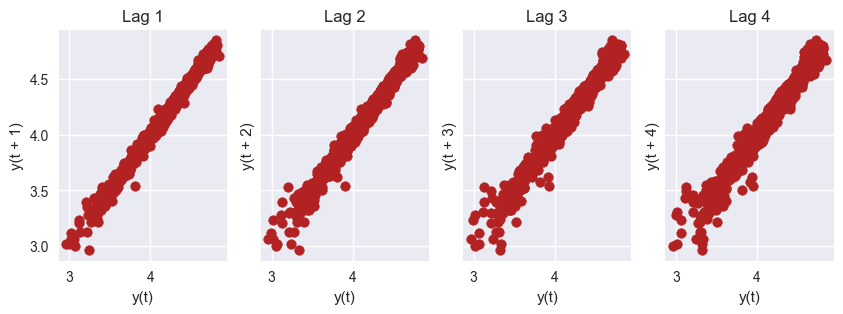
Whilw the original data is non-stationary, the partial autocorrelation function indicates that one order of differentiation is needed to make the series stationary. What we will try to do is to find a value in between 0 and 1 that makes the series stationary but such that the differentiated series is highly correlated with the original data.
fig, axes = plt.subplots(1,2,figsize=(16,3), dpi= 100, sharey=True)
plot_acf(values.tolist(), lags=20, ax=axes[0])
plot_pacf(values.tolist(), lags=20, ax=axes[1])
axes[0].set_ylim(-1.05, 1.05);

The first step is to get the weights for the fractional derivation. This is done by function get_weights() for any given order, up to max_size coefficients and discarding all values that are, in absolute value, below the specified threshold.
def get_weights(d, max_size=10, threshold=1e-5):
    w = [1.0]
    for k in range(1, max_size):
        w.append(-w[-1] / k * (d - k + 1))
        if abs(w[-1]) < threshold:
            break
    return np.array(w[::-1])
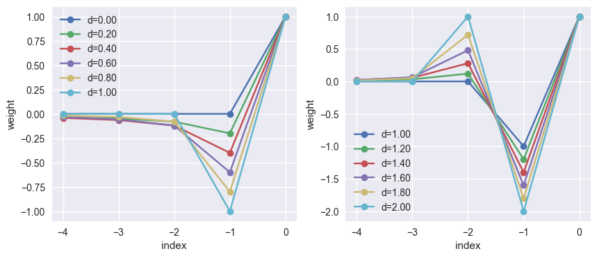
A visual representation of the weights is reported below, using a differentiation order from 0 to 1 on the left and from 1 to 2 on the right. The notable cases of $d=1$ and $d=2$ yield the coefficients of the well-know finite different on uniform grids.
fig, (ax0, ax1) = plt.subplots(figsize=(10, 4), nrows=1, ncols=2)
for d in np.linspace(0, 1, 6):
    ax0.plot([-4, -3, -2, -1, 0], get_weights(d, 5, 0.0), '-o', label=f'd={d:.2f}')
ax0.legend(loc='upper left')

for d in np.linspace(1, 2, 6):
    ax1.plot([-4, -3, -2, -1, 0], get_weights(d, 5, 0.0), '-o', label=f'd={d:.2f}')
ax1.legend(loc='lower left')

for ax in [ax0, ax1]:
    ax.set_xlabel('index')
    ax.set_ylabel('weight')

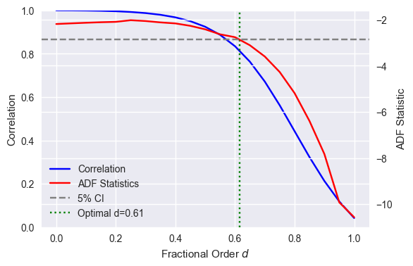
The goal now is to fine the lowest value of $d$ that gives a stationary series. First we run through several values between 0 and 1 for illustration purposed, then we use an nonlinear solver.
adf_all, kpss_all, corr_all = [], [], []
ds = np.linspace(0.0, 1.0, 21)
for d in ds:
    weights = get_weights(d, 10, 0.0)
    X_frac = values.rolling(window=10).apply(lambda x: np.dot(x, weights)).dropna()

    result = adfuller(X_frac, autolag='AIC')
    adf_all.append(result[0])

    X_frac.name = 'frac'
    X2 = pd.concat((values, X_frac), axis=1)
    corr_all.append(X2.corr()['values']['frac'])

    ci_05 = result[4]['5%']
from scipy.optimize import root_scalar
status = root_scalar(lambda x: np.interp(x, ds, adf_all) - ci_05, bracket=[0, 1])
assert status.converged
d_opt = status.root
fig, ax = plt.subplots(figsize=(6, 4))
l1 = ax.plot(ds, corr_all, color='blue', label='Correlation')
ax.set_ylim(0, 1)
ax.set_ylabel('Correlation')
ax2 = ax.twinx()
l2 = ax2.plot(ds, adf_all, color='red', label='ADF Statistics')
l3 = ax2.axhline(y=ci_05, linestyle='dashed', color='grey', label='5% CI')
l4 = ax.axvline(x=d_opt, linestyle='dotted', color='green', label=f'Optimal d={d_opt:.2f}')
lines = l1 + l2 + [l3, l4]
ax.legend(lines, [l.get_label() for l in lines], loc='lower left')
ax2.set_ylabel('ADF Statistic')
ax.set_xlabel('Fractional Order $d$');

This reproduces the graph on Lopez de Prado’s book. Once an optimal value of $d$ is found, it can be used to produce effective features for forecasts.