In this article we go through Gyöngy’s theorem. This result, widely used in mathematical finance, was originally published in Gyöngy, I. (1986). Mimicking the one-dimensional marginal distributions of processes having an Itô differential. Probability Theory and Related Fields, 71(4), 501–516. The theorem addresses a common situation in quantitative finance: your model is multidimensional — it includes stochastic volatility, stochastic interest rates, or other auxiliary factors — but only one coordinate, typically the stock price, appears in option payoffs. Gyöngy’s theorem says that any such multidimensional model can be replaced by a single scalar SDE that has the same one-dimensional marginal distributions at every point in time. Expectations of payoffs are therefore identical in both models. This is the theoretical backbone of Dupire’s local volatility formula: it tells you that, no matter how complex the true dynamics, there always exists a local volatility model that reprices all vanilla options correctly.
Suppose your model consists of a scalar process $X_t \in \mathbb{R}$ — in finance, the (logarithm of the) stock price — and a vector of auxiliary factors $Y_t \in \mathbb{R}^{d-1}$ — for example, stochastic volatility or interest rates. Together they form a coupled system driven by a $d$-dimensional Brownian motion $W_t$:
\[dX_t = \mu(t, X_t, Y_t)\, dt + \sigma(t, X_t, Y_t)\, dW_t\] \[dY_t = \beta(t, X_t, Y_t)\, dt + \gamma(t, X_t, Y_t)\, dW_t\]Here $\mu \in \mathbb{R}$ and $\sigma \in \mathbb{R}^{1 \times d}$ are the drift and diffusion coefficients of $X_t$, while $\beta$ and $\gamma$ are the corresponding objects for $Y_t$. The key difficulty is that $\mu$ and $\sigma$ depend on $Y_t$: the hidden factors influence the dynamics of $X_t$, making the system genuinely multidimensional and hard to work with.
Gyöngy’s result shows that the entire coupled system can be replaced by a single scalar SDE for $X_t$ alone, provided the right coefficients are chosen. Define the local drift and local variance by averaging the coefficients of $X_t$ over the hidden factors, conditional on the current value of $X_t$:
\[\hat\mu(t, x) := \mathbb{E}\!\left[ \mu(t, X_t, Y_t) \mid X_t = x \right]\] \[\hat\sigma^2(t, x) := \mathbb{E}\!\left[ \sigma(t, X_t, Y_t)\, \sigma(t, X_t, Y_t)^\top \mid X_t = x \right]\]Then the mimicking SDE is:
\[d\hat{X}_t = \hat\mu(t, \hat{X}_t)\, dt + \sqrt{\hat\sigma^2(t, \hat{X}_t)}\, d\hat{W}_t\]where $\hat{W}_t$ is a standard one-dimensional Brownian motion. There is no $Y_t$ anywhere. Gyöngy’s theorem states that $\hat{X}_t$ has exactly the same one-dimensional marginal distributions as $X_t$ at every time $t \in [0, T]$: for any bounded measurable $f$,
\[\mathbb{E}[f(X_t)] = \mathbb{E}[f(\hat{X}_t)].\]The strategy is to show that $X_t$ and $\hat{X}_t$ both satisfy the same evolution equation for expectations, then conclude they share the same law by uniqueness.
Step 1 — Probe with a test function
| Pick any $\varphi \in C_c^\infty(\mathbb{R})$ and apply Itô’s formula to $\varphi(X_t)$. Since $X_t$ is a scalar Itô process with drift $\mu(t, X_t, Y_t)$ and instantaneous variance $ | \sigma(t, X_t, Y_t) | ^2 = \sigma \sigma^\top$, taking expectations kills the stochastic integral and gives: |
This is exact, but the right-hand side still involves $Y_t$.
Step 2 — Apply the tower property
Since $\varphi’(X_t)$ is a function of $X_t$ alone, the tower property of conditional expectation gives:
\[\mathbb{E}\!\left[ \varphi'(X_t) \cdot \mu(t, X_t, Y_t) \right] = \mathbb{E}\!\left[ \varphi'(X_t) \cdot \mathbb{E}\!\left[ \mu(t, X_t, Y_t) \mid X_t \right] \right]\]The inner expectation is exactly $\hat\mu(t, X_t)$ — the average drift of $X_t$ given its current value, with $Y_t$ integrated out. Applying the same argument to the variance term, the equation becomes:
\[\partial_t\, \mathbb{E}[\varphi(X_t)] = \mathbb{E}\!\left[ \varphi'(X_t)\, \hat\mu(t, X_t) + \tfrac{1}{2}\, \varphi''(X_t)\, \hat\sigma^2(t, X_t) \right]\]The factors $Y_t$ have been eliminated completely: the right-hand side depends on the process only through $X_t$.
Step 3 — The mimicking SDE satisfies the same equation
Apply Itô’s formula to $\varphi(\hat{X}_t)$ and take expectations. The drift of $\hat{X}_t$ is $\hat\mu(t, \hat{X}_t)$ and its instantaneous variance is $\hat\sigma^2(t, \hat{X}_t)$ by construction, so:
\[\partial_t\, \mathbb{E}[\varphi(\hat{X}_t)] = \mathbb{E}\!\left[ \varphi'(\hat{X}_t)\, \hat\mu(t, \hat{X}_t) + \tfrac{1}{2}\, \varphi''(\hat{X}_t)\, \hat\sigma^2(t, \hat{X}_t) \right]\]This is identical in form to what we derived for $X_t$. The coefficients $\hat\mu$ and $\hat\sigma^2$ were defined precisely so this would hold.
Step 4 — Uniqueness closes the argument
Both $X_t$ and $\hat{X}_t$ start from the same distribution at $t = 0$ and satisfy the same equation for all test functions $\varphi$. This is the martingale problem for the generator:
\[\mathcal{L}_t \varphi(x) = \hat\mu(t, x)\, \varphi'(x) + \tfrac{1}{2}\, \hat\sigma^2(t, x)\, \varphi''(x)\]Under mild regularity on $\hat\mu$ and $\hat\sigma^2$, this problem has a unique solution in the space of probability measures. Both $X_t$ and $\hat{X}_t$ are solutions, so their laws must agree at every $t$. $\blacksquare$
A few remarks are in order. First, the equivalence is not pathwise: $X_t$ and $\hat{X}_t$ need not be close on the same probability space, and in fact the two processes typically live on entirely different spaces. The proof works purely at the level of marginal distributions.
Second, the tower property in Step 2 is the real engine of the argument. It lets you integrate out $Y_t$ without any approximation, replacing the complicated joint dynamics by a single scalar equation. The price is that $\hat\mu$ and $\hat\sigma^2$ are not simple explicit functions — they encode the average effect of the hidden factors on $X_t$, conditional on its current value. Computing them requires knowing the joint law of $(X_t, Y_t)$, which is typically the hard part in practice.
Third, and most importantly for applications: if you already know the local variance function $\hat\sigma^2(t, x)$ — for instance, because you have calibrated it from market option prices via Dupire’s formula — you can write down the mimicking SDE directly, without ever specifying the full multidimensional model. The theorem guarantees that the resulting one-dimensional model will reprice all European payoffs correctly.
The Heston model: a worked example
We apply Gyöngy’s theorem concretely to the Heston stochastic volatility model. The state is $(X_t, V_t)$ where $X_t = \log S_t$ is the log-price and $V_t$ is the instantaneous variance:
\[dX_t = \left(r - \frac{V_t}{2}\right)dt + \sqrt{V_t}\,dW_t^S, \qquad dV_t = \kappa(\theta - V_t)\,dt + \xi\sqrt{V_t}\,dW_t^V\]with $\langle dW_t^S, dW_t^V \rangle = \rho\,dt$. We use the parameters $r = 0.05$, $\kappa = 2.0$, $\theta = 0.04$ (long-run variance, i.e. long-run vol of 20%), $\xi = 0.3$ (vol-of-vol), $\rho = -0.7$, $V_0 = \theta$. The Feller condition $2\kappa\theta \geq \xi^2$, which ensures $V_t$ stays strictly positive almost surely, is satisfied: $0.16 \geq 0.09$.
The Gyöngy projection in Heston
Writing the correlated drivers in terms of two independent Brownians ($dW_t^V = dW_t^1$, $dW_t^S = \rho\,dW_t^1 + \sqrt{1-\rho^2}\,dW_t^2$), the diffusion matrix of $(X_t, V_t)$ is:
\[A = \begin{pmatrix} v & \rho\xi v \\ \rho\xi v & \xi^2 v \end{pmatrix}\]The instantaneous variance of $X_t$ is $A_{11} = V_t$, so the Gyöngy local variance and local drift are:
\[\hat\sigma^2(t, x) = \mathbb{E}[V_t \mid X_t = x], \qquad \hat\mu(t, x) = r - \tfrac{1}{2}\hat\sigma^2(t, x)\]Both are determined by the same conditional expectation. The mimicking SDE is:
\[d\hat{X}_t = \left(r - \tfrac{\hat\sigma^2(t, \hat{X}_t)}{2}\right)dt + \hat\sigma(t, \hat{X}_t)\,d\hat{W}_t\]This is precisely the Dupire local volatility model calibrated to the Heston marginals.
Fokker-Planck equation for the joint density
The joint density $p(t, x, v)$ of $(X_t, V_t)$ evolves according to the Fokker-Planck equation:
\[\partial_t p = -\partial_x\!\left[\!\left(r - \tfrac{v}{2}\right)p\right] - \partial_v\!\left[\kappa(\theta-v)\,p\right] + \tfrac{1}{2}\partial_{xx}(vp) + \rho\xi\,\partial_{xv}(vp) + \tfrac{\xi^2}{2}\partial_{vv}(vp)\]with initial condition $p(0, x, v) = \delta(x - X_0)\,\delta(v - V_0)$.
Numerical procedure
We solve this PDE on a uniform $(x, v)$ grid using an explicit finite-difference scheme in conservation form. Each term is discretized as a central difference of the corresponding flux. The time step is chosen to satisfy the CFL conditions for all three diffusion operators (x-diffusion, v-diffusion, and cross term). At each snapshot time $t$, we integrate out $v$ numerically:
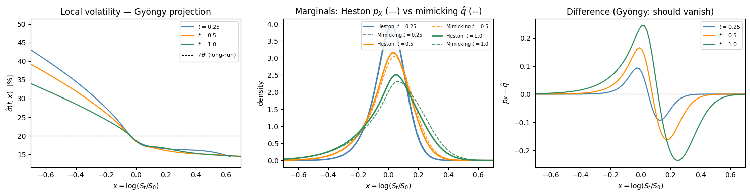
\[p_X(t, x) = \int_0^\infty p(t, x, v)\,dv, \qquad \hat\sigma^2(t, x) = \frac{\displaystyle\int_0^\infty v\,p(t, x, v)\,dv}{p_X(t, x)}\]The resulting surface $\hat\sigma^2(t, x)$ is the local variance of the Gyöngy mimicking process.
import numpy as np
import matplotlib.pyplot as plt

# --- Heston parameters ---
r, kappa, theta, xi, rho = 0.05, 2.0, 0.04, 0.3, -0.7
V0, X0, T = theta, 0.0, 1.0

print(f"Feller: 2κθ = {2*kappa*theta:.3f} ≥ ξ² = {xi**2:.3f}  ✓")

# --- Spatial grid ---
Nx, Nv = 120, 70
x = np.linspace(-1.0, 1.0, Nx)
v = np.linspace(1e-5, 0.50, Nv)
dx, dv = x[1] - x[0], v[1] - v[0]
X2d, V2d = np.meshgrid(x, v, indexing='ij')   # shape (Nx, Nv)

# --- Initial densities: narrow Gaussian centred on (X0, V0) ---
p = np.exp(-((X2d - X0)**2 / (3*dx)**2 + (V2d - V0)**2 / (3*dv)**2) / 2)
p /= p.sum() * dx * dv
q = p.sum(axis=1) * dv   # 1D mimicking density: same initial marginal in x

# --- Time step from CFL conditions ---
v_max = v.max()
dt = 0.2 * min(
    dx**2 / v_max,                         # ½∂_xx(vp)
    dv**2 / (xi**2 * v_max),              # ½∂_vv(ξ²vp)
    dx * dv / (abs(rho) * xi * v_max),    # ∂_xv(ρξvp)
)
Nt = int(np.ceil(T / dt));  dt = T / Nt
print(f"dt = {dt:.2e},  steps = {Nt:,}")

# --- Snapshot storage ---
snap_times = [0.25, 0.5, 1.0]
local_var, marginal_px, mimicking_px = {}, {}, {}

# --- Combined 2D (Heston) + 1D (mimicking) explicit FD loop ---
for n in range(Nt):

    # ── 2D Fokker-Planck for (X_t, V_t) ──────────────────────────────────
    ap = (r - V2d / 2) * p
    Lx = np.zeros_like(p)
    Lx[1:-1, :] = -(ap[2:, :] - ap[:-2, :]) / (2 * dx)

    bp = kappa * (theta - V2d) * p
    Lv = np.zeros_like(p)
    Lv[:, 1:-1] = -(bp[:, 2:] - bp[:, :-2]) / (2 * dv)

    vp  = V2d * p
    Dxx = np.zeros_like(p)
    Dxx[1:-1, :] = 0.5 * (vp[2:, :] - 2*vp[1:-1, :] + vp[:-2, :]) / dx**2

    evp = xi**2 * V2d * p
    Dvv = np.zeros_like(p)
    Dvv[:, 1:-1] = 0.5 * (evp[:, 2:] - 2*evp[:, 1:-1] + evp[:, :-2]) / dv**2

    dvp = rho * xi * V2d * p
    Dxv = np.zeros_like(p)
    Dxv[1:-1, 1:-1] = (
        dvp[2:, 2:] - dvp[2:, :-2] - dvp[:-2, 2:] + dvp[:-2, :-2]
    ) / (4 * dx * dv)

    p  = p + dt * (Lx + Lv + Dxx + Dvv + Dxv)
    p  = np.maximum(p, 0.0)
    p /= p.sum() * dx * dv

    # ── Local variance from marginalising the 2D density ─────────────────
    p_X = p.sum(axis=1) * dv                   # marginal density of X_t
    sv2 = np.where(
        p_X > 1e-8 * p_X.max(),
        (V2d * p).sum(axis=1) * dv / p_X,      # E[V_t | X_t = x]
        theta,                                   # fall back to θ in the tails
    )

    # ── 1D Fokker-Planck for the mimicking process X̂_t ───────────────────
    # ∂_t q = −∂_x[(r − σ̂²/2) q] + ½∂_xx(σ̂² q)
    aq = (r - sv2 / 2) * q
    Lq = np.zeros_like(q)
    Lq[1:-1] = -(aq[2:] - aq[:-2]) / (2 * dx)

    sv2q = sv2 * q
    Dq   = np.zeros_like(q)
    Dq[1:-1] = 0.5 * (sv2q[2:] - 2*sv2q[1:-1] + sv2q[:-2]) / dx**2

    q  = q + dt * (Lq + Dq)
    q  = np.maximum(q, 0.0)
    q /= q.sum() * dx

    # ── Snapshots ─────────────────────────────────────────────────────────
    t_now = (n + 1) * dt
    for t_s in snap_times:
        if abs(t_now - t_s) < 0.5 * dt:
            p_X_s = p.sum(axis=1) * dv
            sv2_s = np.where(p_X_s > 1e-8 * p_X_s.max(),
                             (V2d * p).sum(axis=1) * dv / p_X_s, np.nan)
            local_var[t_s]    = sv2_s.copy()
            marginal_px[t_s]  = p_X_s.copy()
            mimicking_px[t_s] = q.copy()

print("Done.")
Feller: 2κθ = 0.160 ≥ ξ² = 0.090  ✓
dt = 1.13e-04,  steps = 8,851
Done.
fig, axes = plt.subplots(1, 3, figsize=(15, 4))
colors = ['steelblue', 'darkorange', 'seagreen']

# ── Panel 1: Local volatility surface ────────────────────────────────────
ax = axes[0]
for t_s, col in zip(snap_times, colors):
    ax.plot(x, 100 * np.sqrt(local_var[t_s]), color=col, label=f'$t = {t_s}$')
ax.axhline(100 * np.sqrt(theta), color='k', ls='--', lw=0.8, label=r'$\sqrt{\theta}$ (long-run)')
ax.set_xlabel(r'$x = \log(S_t/S_0)$')
ax.set_ylabel(r'$\hat\sigma(t,x)$  [%]')
ax.set_title('Local volatility — Gyöngy projection')
ax.set_xlim(-0.7, 0.7)
ax.legend(fontsize=8)

# ── Panel 2: Marginal densities — Heston vs mimicking ────────────────────
ax = axes[1]
for t_s, col in zip(snap_times, colors):
    ax.plot(x, marginal_px[t_s],  color=col, lw=2.0,       label=f'Heston  $t={t_s}$')
    ax.plot(x, mimicking_px[t_s], color=col, lw=1.2, ls='--', label=f'Mimicking $t={t_s}$')
ax.set_xlabel(r'$x = \log(S_t/S_0)$')
ax.set_ylabel(r'density')
ax.set_title(r'Marginals: Heston $p_X$ (—) vs mimicking $\hat{q}$ (--)')
ax.set_xlim(-0.7, 0.7)
ax.legend(fontsize=7, ncol=2)

# ── Panel 3: Pointwise difference ────────────────────────────────────────
ax = axes[2]
for t_s, col in zip(snap_times, colors):
    diff = marginal_px[t_s] - mimicking_px[t_s]
    ax.plot(x, diff, color=col, label=f'$t = {t_s}$')
ax.axhline(0, color='k', lw=0.8, ls='--')
ax.set_xlabel(r'$x = \log(S_t/S_0)$')
ax.set_ylabel(r'$p_X - \hat{q}$')
ax.set_title('Difference (Gyöngy: should vanish)')
ax.set_xlim(-0.7, 0.7)
ax.legend(fontsize=8)

plt.tight_layout()
plt.show()
Conclusions
Gyöngy’s theorem is a universality result: whatever the internal complexity of a multidimensional model, its marginal distributions at each time $t$ can always be reproduced exactly by a scalar SDE. For option pricing this means that every multidimensional model has a one-dimensional shadow — a local volatility model — that prices all European payoffs identically. Dupire’s formula is the most famous instance, but the theorem applies far more broadly.
A few things are worth keeping in mind when using the theorem in practice.
What is preserved and what is not. The projection preserves one-dimensional marginals: the distribution of $X_t$ at each fixed $t$. It does not preserve the joint distribution of $(X_s, X_t)$ for $s \neq t$. As a result, the mimicking process and the original model agree on all European payoffs but can disagree substantially on path-dependent ones: barriers, Asians, lookbacks, and cliquets all see through the projection and depend on the full multidimensional dynamics.
Two models, one local vol surface. The theorem is a many-to-one map: many different multidimensional models can share the same local volatility surface. This is why calibrating a local vol model to vanilla option prices does not identify the true dynamics — it only identifies the marginals. Distinguishing between models that share the same local vol requires path-dependent instruments.
Numerical methods. For two-dimensional models the Fokker–Planck PDE on a $(x, v)$ grid is effective and accurate. The local variance is extracted at every time step as a ratio of two marginal integrals, and the 1D mimicking density can be advanced simultaneously at negligible extra cost. For higher-dimensional models the PDE becomes intractable and Monte Carlo with kernel regression is the natural alternative: simulate the full system, estimate the conditional expectation at each step via Nadaraya–Watson, and feed the result into the 1D Fokker–Planck.