The Heston model is given by the following equations in a risk-neutral measure
\[\begin{aligned} \frac{dS(t)}{S(t)} & =\mu dt + \sqrt{V(t)} dW_S(t) \\ dV(t) & = \kappa(\theta−V(t)) dt + \zeta \sqrt{V(t)} dW_V(t) \\ < dW_S(t), dW_V(t)> & =ρdt, \end{aligned}\]with $\mu = r - q$.
It is easy to see that the process for the inverted spot $U(t) = S(t)^{-1}$ is still described by the Heston model. Using Itô’s lemma on $U(t) = f(S(t))$, with
\[\begin{aligned} f(s) & = \frac{1}{s} \\ % f'(s) & = -\frac{1}{s^2} \\ % f''(s) & = \frac{2}{s^3}, \\ \end{aligned}\]gives
\[dU(t) = \left( -\mu S(t) \frac{1}{S(t)^2} + \frac{1}{2} V(t) S(t)^2 \frac{2}{S(t)^3} \right)dt - \sqrt{V(t)}S(t)\frac{1}{S(t)^2} dW_S(t)\]and therefore
\[\frac{dU(t)}{U(t)} = \left( -\mu + V(t) \right) dt - \sqrt{V(t)}dW_S(t).\]We can change the measure by using
\[dW_U(t) = -dW_S(t) + \sqrt{V(t)} dt\]such that the appropriately discounted spot process becomes a martingale. We still need to adjust the second process as $dW_S(t)$ and $dW_V(t)$ are correlated. To do that, we first use
\[dW_V(t) = \rho dW_S(t) + \sqrt{1 - \rho^2} dW_V^\perp(t),\]where $dW_S(t)$ and $dW_V^\perp(t)$ are independent, then use our definition of $dW_U(t)$ above to obtain
\[dW_V(t) = - \rho dW_U(t) + \rho\sqrt{V(t)}dt + \sqrt{1 - \rho^2} dW_V^\perp(t)\]such that
\[\begin{aligned} dV(t) & = \kappa(\theta - V(t))dt + \zeta \sqrt{V(t)} dW_V(t) \\ % & = \kappa(\theta - V(t))dt + \zeta \sqrt{V(t)} \left( -\rho dW_U(t) + \rho \sqrt{V(t)} dt + \sqrt{1 - \rho^2} dW_V^\perp(t) \right) \\ % & = \kappa \theta dt - \kappa V(t) dt + \zeta \rho V(t) dt + \zeta \sqrt{V(t)}\left( -\rho dW_U(t) + \sqrt{1 - \rho^2} dW_V^\perp(t) \right) \\ % & = \left( \kappa \theta - (\kappa - \zeta \rho) V(t) \right) dt + \zeta \sqrt{V(t)} dW_{\bar{V}}(t) \\ % & = (\kappa \theta - \bar\kappa V(t)) dt + \zeta \sqrt{V(t)} dW_{\bar{V}}(t) \\ % & = \bar\kappa \left( \frac{\kappa}{\bar\kappa}\theta - V(t) \right) dt + \zeta \sqrt{V(t)} dW_{\bar{V}}(t) \\ % & = \bar\kappa(\bar\theta - V(t)) dt + \zeta \sqrt{V(t)} dW_{\bar{V}}(t), \end{aligned}\]with
\[\begin{aligned} <dW_U(t), dW_{\bar{V}}(t)> & = -\rho dt \\ % \bar\kappa & = \kappa - \zeta \rho \\ % \bar\theta & = \frac{\kappa}{\bar \kappa} \theta. \end{aligned}\]Clearly, if $\rho = 0$, we just have $\bar\kappa = \kappa$, $\bar\theta = \theta$, meaning that in this case the $V(t)$ process is unchanged.
from dataclasses import dataclass
import matplotlib.colors as mcolors
import matplotlib.pylab as plt
from mpl_toolkits.mplot3d.axes3d import Axes3D
import numpy as np
import scipy.integrate
from scipy.optimize import root_scalar
from scipy.stats import norm
Φ = norm.cdf
The Contract class wraps the basic ingredients of a vanilla contract – the maturity T, the strike K, and a boolean flag to indicate whether it is a call or a put.
@dataclass
class Contract:
    K: float
    T: float
    is_call: bool
The Model class defines a Heston model and provides the methods to price a vanilla contract with the closed-form approximation and Monte Carlo. The closed-form approximation requires the numerical integration of an indefinite integral, done using scipy.integrate.quad_vec, while for Monte Carlo pricing we first generate a number of paths with the Heston dynamics and then evaluate in expectation the value of the vanilla payoff at expiry (which is then discounted to time 0).
@dataclass
class Model:
    S_0: float
    r: float
    q: float
    V_0: float
    κ: float
    θ: float
    ζ: float
    ρ: float

    def __str__(self):
        return f'S_0={self.S_0}, V_0={self.V_0}, κ={self.κ}, θ={self.θ}, ζ={self.ζ}, ρ={self.ρ}'

    def phi(self, u, tau):
        alpha_hat = -0.5 * u * (u + 1j)
        beta = self.κ - 1j * u * self.ζ * self.ρ
        gamma = 0.5 * self.ζ ** 2
        d = np.sqrt(beta**2 - 4 * alpha_hat * gamma)
        g = (beta - d) / (beta + d)
        h = np.exp(-d*tau)
        A_ = (beta-d)*tau - 2*np.log((g*h-1) / (g-1))
        A = self.κ * self.θ / (self.ζ**2) * A_
        B = (beta - d) / (self.ζ**2) * (1 - h) / (1 - g*h)
        return np.exp(A + B * self.V_0)

    def integral(self, K, T):
        integrand = (lambda u:
            np.real(np.exp((1j*u + 0.5)*K)*self.phi(u - 0.5j, T))/(u**2 + 0.25))

        i, _ = scipy.integrate.quad_vec(integrand, 0, np.inf)
        return i

    def compute_forward(self, T):
        return self.S_0 * np.exp((self.r - self.q) * T)

    def compute_price(self, contract: Contract):
        K, T = contract.K, contract.T
        a = np.log(self.S_0 / K) + (self.r-self.q) * T
        i = self.integral(a, T)
        call_price = self.S_0 * np.exp(-self.q * T) - K * np.exp(-self.r * T) / np.pi*i
        if contract.is_call:
            return call_price
        else:
            F = np.exp((self.r - self.q) * T) * self.S_0
            return call_price - np.exp(-self.r * T) * (F - K)

    def generate_paths(self, schedule, num_paths):
        num_steps = len(schedule) - 1
        S_all, V_all = [np.ones((num_paths,)) * self.S_0], [np.ones((num_paths,)) * self.V_0]
        X = np.log(S_all[0])
        V = V_all[0]
        W_X = np.random.randn(num_steps, num_paths)
        W_V_ortho = np.random.randn(num_steps, num_paths)
        W_V = self.ρ * W_X + np.sqrt(1 - self.ρ**2) * W_V_ortho

        for i in range(num_steps):
            Δt = schedule[i + 1] - schedule[i]
            sqrt_Δt = np.sqrt(Δt)
            X = X + (self.r - self.q - 0.5 * V) * Δt + np.sqrt(V) * sqrt_Δt * W_X[i]
            V = V + self.κ * (self.θ - V) * Δt + self.ζ * np.sqrt(V) * sqrt_Δt * W_V[i]
            V = np.maximum(V, 0)
            S_all.append(np.exp(X))
            V_all.append(V)

        return np.vstack(S_all), np.vstack(V_all)

    def compute_mc_price(self, S_T, contract: Contract):
        df = np.exp(-self.r * contract.T)
        ω = 1.0 if contract.is_call else -1.0
        Π = df * np.maximum(ω * (S_T - contract.K), 0)
        mc_price, mc_std = Π.mean(), Π.std() / np.sqrt(len(S_T))
        return mc_price, mc_std
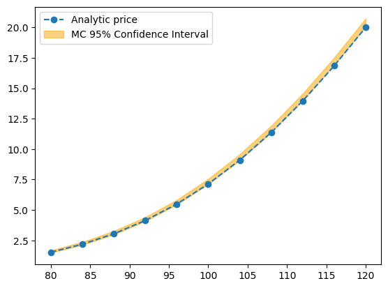
We compare the closed-form prices with the ones given by the Monte Carlo method as a check.
model = Model(S_0=100.0, r=0.02, q=0.01, V_0=0.04, κ=1.0, θ=0.04, ζ=0.2, ρ=-0.8)
K_all = np.linspace(0.8 * model.S_0, 1.2 * model.S_0, 11)
S_all = None
analytic_prices, mc_lower_prices, mc_upper_prices = [], [], []
for K in K_all:
    contract = Contract(K, 1.0, False)
    if S_all is None:
        S_all, _ = model.generate_paths(np.linspace(0, contract.T, 201), 10_000)
    analytic_prices.append(model.compute_price(contract))
    mc_price, mc_std_dev = model.compute_mc_price(S_all[-1], contract)
    mc_lower_prices.append(mc_price - 1.96 * mc_std_dev)
    mc_upper_prices.append(mc_price + 1.96 * mc_std_dev)
plt.plot(K_all, analytic_prices, '--o', label='Analytic price')
plt.fill_between(K_all, mc_lower_prices, mc_upper_prices, alpha=0.5, color='orange', label='MC 95% Confidence Interval')
plt.legend();
It is customary to quote vanilla prices using implied volatilities, that is the volatility that is required by the Black-Scholes formula in order to generate the same price. This means that we use closed-form approximation above to compute the Heston price, then with a root search algorithm we compute the implied volatility. The procedure is repeated over several strikes and maturities and gives rise to the so-called volatility surface.
def compute_black_scholes_price(S_0, r, q, σ, contract):
    K, T, is_call = contract.K, contract.T, contract.is_call
    ω = 1.0 if is_call else -1.0
    if T == 0.0:
        return max(ω * (S_0 - K), 0.0)
    df = np.exp(-r * T)
    F = S_0 * np.exp((r - q) * T)
    d_plus = (np.log(F / K) + 0.5 * σ**2 * T) / σ / np.sqrt(T)
    d_minus = d_plus - σ * np.sqrt(T)
    return ω * df * (F * Φ(ω * d_plus) - K * Φ(ω * d_minus))
def compute_implied_vol(S_0, r, q, σ_0, contract, target_price):
    def inner(σ):
        return compute_black_scholes_price(S_0, r, q, σ, contract) - target_price
    try:
        result = root_scalar(inner, x0=σ_0, bracket=[1e-3, 0.5])
    except:
        return np.nan
    return np.nan if not result.converged else result.root
def compute_smile(model, T, factor=3, num_points=101):
    F = model.compute_forward(T)
    contract = Contract(K=F, T=T, is_call=True)
    price_ATM = model.compute_price(contract)
    σ_ATM = compute_implied_vol(model.S_0, model.r, model.q, 0.5, contract, price_ATM)
    width = factor * σ_ATM * np.sqrt(T)

    σs = []
    Ks = np.linspace(F * np.exp(-width), F * np.exp(width), num_points)
    for K in Ks:
        contract = Contract(K=K, T=T, is_call=K > F)
        price = model.compute_price(contract)
        σ = compute_implied_vol(model.S_0, model.r, model.q, 0.5, contract, price)
        σs.append(σ)

    return Ks, σs
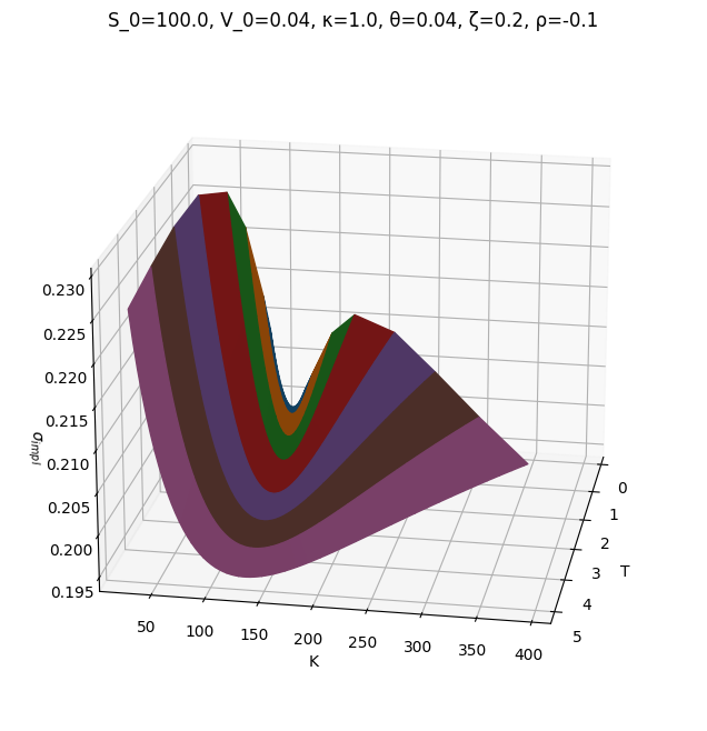
We plot the volatility surface using a 3D plot, with strikes on the X-axis, maturities on the Y-axis, and the implied volatility itself on the Z-axis.
X, Y, Z, C = [], [], [], []
colors = list(mcolors.TABLEAU_COLORS.values())
model = Model(S_0=100.0, r=0.02, q=0.01, V_0=0.04, κ=1.0, θ=0.04, ζ=0.2, ρ=-0.1)
for color, T in zip(colors, [1 / 12, 2 / 12, 6 / 12, 1, 2, 3, 4, 5]):
    Ks, σs = compute_smile(model, T)
    X.append([T] * len(Ks))
    Y.append(Ks)
    Z.append(σs)
    C.append([color] * len(Ks))
fig, ax = plt.subplots(subplot_kw={'projection': '3d'}, figsize=(8, 8))
ax.plot_surface(np.array(X), np.array(Y), np.array(Z), facecolors=C)
ax.view_init(elev=20, azim=10, roll=0)
ax.set_xlabel('T')
ax.set_ylabel('K')
ax.set_zlabel('$σ_{impl}$')
ax.set_title(model);
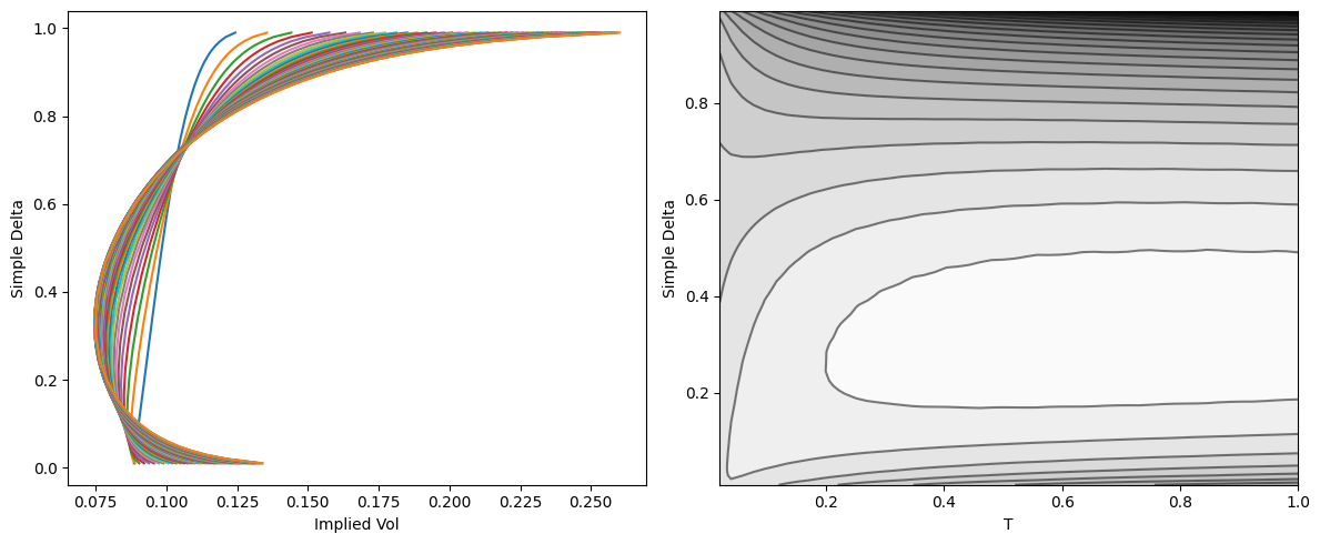
The picture above is nice yet a bit difficult to interpret, and often without convenient view angles can be confusing. A better way is to replace strikes with the so-called simple delta, defined as
\[\delta_{simple}(K, T) = \Phi\left( \frac{\log(F / K)}{\sigma \sqrt{T}} \right),\]where $\Phi$ is the cumulative density function of the normal distribution, $T$ the maturity of the option, $F$ the forward at $T$, and $K$ the strike. By definition $\delta_{simple}$ is a number between 0 and 1 for all maturities and gives a convenient way of adimensionalize the moneyness $F/K$. One such surface is computed below.
def compute_vol_on_delta_grid(T, d_grid, num_points):
    F = model.compute_forward(T)
    Ks, σs = compute_smile(model, T, factor=9, num_points=num_points)
    ds = Φ(np.log(Ks / F) / σs / np.sqrt(T))
    σs = np.interp(d_grid, ds, σs)
    # remove nans at the extremes, replace them with flat interpolation
    n = len(σs)
    for i in range(n // 2, 0, -1):
        if np.isnan(σs[i - 1]):
            σs[i - 1] = σs[i]
    for i in range(n // 2, n - 1):
        if np.isnan(σs[i + 1]):
            σs[i + 1] = σs[i]
    return σs
model = Model(S_0=1.0, r=0.05, q=0.03, V_0=0.1**2, κ=0.25, θ=0.2**2, ζ=0.5, ρ=-0.5)
d_grid = np.linspace(0.01, 0.99, 101)
X, Y, Z = [], [], []
T_all = [m / 52 for m in range(1, 53)]
for T in T_all:
    σs = compute_vol_on_delta_grid(T, d_grid, 101)
    X.append([T] * len(σs))
    Y.append(d_grid)
    Z.append(σs)
fig, (ax0, ax1) = plt.subplots(figsize=(12, 5), ncols=2)
for y, z in zip(Y, Z):
    ax0.plot(z, y)
ax0.set_xlabel('Implied Vol'); ax0.set_ylabel('Simple Delta')
ax1.contour(X, Y, Z, colors='k', levels=25, alpha=0.5)
ax1.contourf(X, Y, Z, cmap='binary', levels=25)
ax1.set_xlabel('T'); ax1.set_ylabel('Simple Delta')
fig.tight_layout()