Danie Krige was a South African mining engineer faced with a practical problem: given gold assay measurements at a handful of borehole locations, how do you estimate ore grades at unsampled points in a reef? Errors in either direction are costly — underestimating leads to missing profitable ore, overestimating leads to unprofitable extraction. Accuracy matters, but so does knowing how much to trust the estimate.
Krige’s 1951 master’s thesis proposed a solution based on the statistical structure of the ore grade field itself. Georges Matheron later gave the method its theoretical foundation in the 1960s, coining the name kriging and embedding it in the framework of geostatistics. From a modern statistical perspective, kriging is equivalent to Gaussian Process Regression (GPR): the unknown function is modeled as a sample from a Gaussian process, and predictions follow from Bayesian conditioning on the observed data.
Let’s start from the mathematical framework. Let $\mathcal{D} = {(\mathbf{x}i, y_i)}{i=1}^n$ be a set of $n$ observations, where
\[\mathbf{x}_i \in \mathbb{R}^d\]are input locations and $y_i \in \mathbb{R}$ are output values. We model the underlying function $f$ as a Gaussian process,
\[f(\mathbf{x}) \sim \mathcal{GP}(0,\, k(\mathbf{x}, \mathbf{x}')).\]This means that any finite collection of function values
\[(f(\mathbf{x}_1), \ldots, f(\mathbf{x}_n))^\top\]is jointly Gaussian with covariance matrix
\[K_{ij} = k(\mathbf{x}_i, \mathbf{x}_j).\]The covariance kernel $k(\cdot, \cdot)$ encodes prior beliefs about the smoothness and structure of $f$.
Given training data $(\mathbf{X}, \mathbf{y})$ and a test point $\mathbf{x}^\star$, the joint prior is:
\[\begin{pmatrix} \mathbf{y} \\ f(\mathbf{x}^\star) \end{pmatrix} \sim \mathcal{N}\!\left(\mathbf{0},\, \begin{pmatrix} K(\mathbf{X},\mathbf{X}) + \sigma_n^2 I & \mathbf{k}(\mathbf{X}, \mathbf{x}^\star) \\ \mathbf{k}(\mathbf{x}^\star, \mathbf{X}) & k(\mathbf{x}^\star, \mathbf{x}^\star) \end{pmatrix}\right),\]where $\sigma_n^2$ accounts for observation noise. Conditioning on $\mathbf{y}$ yields $f(\mathbf{x}^\star) \mid \mathbf{y} \sim \mathcal{N}(\mu^\star, {\sigma^\star}^2)$ with:
\[\mu^\star = \mathbf{k}(\mathbf{x}^\star, \mathbf{X})\, \bigl[K + \sigma_n^2 I\bigr]^{-1} \mathbf{y}\] \[{\sigma^\star}^2 = k(\mathbf{x}^\star, \mathbf{x}^\star) - \mathbf{k}(\mathbf{x}^\star, \mathbf{X})\, \bigl[K + \sigma_n^2 I\bigr]^{-1} \mathbf{k}(\mathbf{X}, \mathbf{x}^\star).\]The mean $\mu^\star$ is the kriging estimate; $\sigma^\star$ is its standard deviation and gives a principled measure of uncertainty. When $\sigma_n^2 = 0$ (noise-free interpolation), predictions pass exactly through the training points.
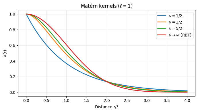
The kernel $k(\mathbf{x}, \mathbf{x}’)$ is the central design choice in kriging. It controls the smoothness of the interpolated surface through its behaviour as a function of distance $r = |\mathbf{x} - \mathbf{x}’|$.
The Matérn family is the most widely used class of kernels in practice. It is parameterized by a smoothness parameter $\nu > 0$ and a length scale $\ell > 0$:
\[k_\nu(r) = \frac{2^{1-\nu}}{\Gamma(\nu)}\left(\frac{\sqrt{2\nu}\, r}{\ell}\right)^\nu K_\nu\!\left(\frac{\sqrt{2\nu}\, r}{\ell}\right)\]where $K_\nu$ is the modified Bessel function of the second kind. For half-integer $\nu$ this simplifies to closed form:
| $\nu$ | $k_\nu(r)$ | Differentiability of $f$ |
|---|---|---|
| $\tfrac{1}{2}$ | $\exp(-r/\ell)$ | $C^0$ |
| $\tfrac{3}{2}$ | $\left(1 + \frac{\sqrt{3}\,r}{\ell}\right)\exp!\left(-\frac{\sqrt{3}\,r}{\ell}\right)$ | $C^2$ |
| $\tfrac{5}{2}$ | $\left(1 + \frac{\sqrt{5}\,r}{\ell} + \frac{5r^2}{3\ell^2}\right)\exp!\left(-\frac{\sqrt{5}\,r}{\ell}\right)$ | $C^4$ |
| $\infty$ | $\exp(-r^2/2\ell^2)$ (RBF) | $C^\infty$ |
The length scale $\ell$ controls the correlation range: small $\ell$ allows rapid local variation, large $\ell$ enforces global smoothness.
import numpy as np
import matplotlib.pyplot as plt
from scipy.spatial.distance import cdist

def matern(r, ell=1.0, nu=1.5):
    r = np.asarray(r, dtype=float) / ell
    if nu == 0.5:
        return np.exp(-r)
    elif nu == 1.5:
        s = np.sqrt(3) * r
        return (1 + s) * np.exp(-s)
    elif nu == 2.5:
        s = np.sqrt(5) * r
        return (1 + s + s**2 / 3) * np.exp(-s)
    else:  # RBF (nu -> inf)
        return np.exp(-0.5 * r**2)

r = np.linspace(0, 4, 300)

fig, ax = plt.subplots(figsize=(7, 4))
for nu, label in [(0.5, r'$\nu=1/2$'), (1.5, r'$\nu=3/2$'), (2.5, r'$\nu=5/2$'), (np.inf, r'$\nu\to\infty$ (RBF)')]:
    ax.plot(r, matern(r, nu=nu), lw=2, label=label)

ax.set_xlabel('Distance $r / \\ell$')
ax.set_ylabel('$k(r)$')
ax.set_title('Matérn kernels ($\\ell = 1$)')
ax.legend()
ax.grid(True, alpha=0.3)
plt.tight_layout()
plt.show()
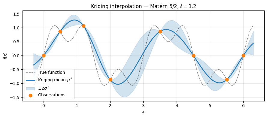
To build intuition we start with one dimension. We implement kriging directly from the predictive equations, using the Matérn $\nu = 5/2$ kernel.
The key implementation detail is the Cholesky decomposition of $K + \sigma_n^2 I$. This is the standard numerically stable approach: instead of inverting the matrix explicitly, we solve the triangular systems $L \alpha = \mathbf{y}$ and $L^\top \boldsymbol{\alpha} = \boldsymbol{\alpha}$, then compute $\mu^\star = \mathbf{k}_*^\top \boldsymbol{\alpha}$.
We observe the function $f(x) = \sin(2\pi x/3) + 0.5\sin(2\pi x)$ at $n = 8$ scattered points.
def matern52(X1, X2, ell=1.0):
    dist = cdist(X1.reshape(-1, 1), X2.reshape(-1, 1))
    r = dist / ell
    return (1 + np.sqrt(5) * r + 5 * r**2 / 3) * np.exp(-np.sqrt(5) * r)

def gp_predict(X_train, y_train, X_test, kernel_fn, noise=1e-8):
    K = kernel_fn(X_train, X_train) + noise * np.eye(len(X_train))
    k_s  = kernel_fn(X_test, X_train)
    k_ss = np.diag(kernel_fn(X_test, X_test))
    L = np.linalg.cholesky(K)
    alpha = np.linalg.solve(L.T, np.linalg.solve(L, y_train))
    mu    = k_s @ alpha
    v     = np.linalg.solve(L, k_s.T)
    sigma = np.sqrt(np.maximum(k_ss - np.sum(v**2, axis=0), 0))
    return mu, sigma

f = lambda x: np.sin(2 * np.pi * x / 3) + 0.5 * np.sin(2 * np.pi * x)

X_train = np.array([0.0, 0.5, 1.2, 2.0, 3.5, 4.5, 5.5, 6.0])
y_train = f(X_train)
X_test  = np.linspace(-0.3, 6.3, 300)

kernel = lambda X1, X2: matern52(X1, X2, ell=1.2)
mu, sigma = gp_predict(X_train, y_train, X_test, kernel)

fig, ax = plt.subplots(figsize=(9, 4))
ax.plot(X_test, f(X_test), 'k--', lw=1.2, alpha=0.5, label='True function')
ax.plot(X_test, mu, 'C0', lw=2, label='Kriging mean $\\mu^*$')
ax.fill_between(X_test, mu - 2*sigma, mu + 2*sigma, alpha=0.2, color='C0', label='$\\pm 2\\sigma^*$')
ax.scatter(X_train, y_train, color='C1', zorder=5, s=60, label='Observations')
ax.set_xlabel('$x$')
ax.set_ylabel('$f(x)$')
ax.set_title('Kriging interpolation — Matérn $5/2$, $\\ell = 1.2$')
ax.legend()
ax.grid(True, alpha=0.3)
plt.tight_layout()
plt.show()
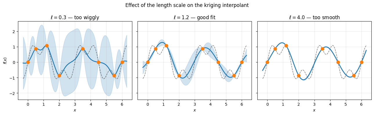
The length scale $\ell$ controls how quickly correlations decay with distance. It is the most influential hyperparameter: a short $\ell$ allows the function to vary rapidly and fit local features; a long $\ell$ enforces a slowly varying, globally smooth interpolant.
In practice, $\ell$ is estimated by maximizing the log marginal likelihood:
\[\log p(\mathbf{y} \mid \mathbf{X}, \boldsymbol{\theta}) = -\tfrac{1}{2}\mathbf{y}^\top K_\theta^{-1} \mathbf{y} - \tfrac{1}{2}\log|K_\theta| - \tfrac{n}{2}\log 2\pi\]This objective automatically penalizes both underfitting (poor data fit) and overfitting (large model complexity), acting as a built-in Occam’s razor. The three panels below show the same eight observations fitted with three different length scales.
fig, axes = plt.subplots(1, 3, figsize=(13, 4), sharey=True)

settings = [
    (0.3, '$\\ell = 0.3$ — too wiggly'),
    (1.2, '$\\ell = 1.2$ — good fit'),
    (4.0, '$\\ell = 4.0$ — too smooth'),
]

for ax, (ell, title) in zip(axes, settings):
    kernel = lambda X1, X2, ell=ell: matern52(X1, X2, ell=ell)
    mu, sigma = gp_predict(X_train, y_train, X_test, kernel)
    ax.plot(X_test, f(X_test), 'k--', lw=1.2, alpha=0.5)
    ax.plot(X_test, mu, 'C0', lw=2)
    ax.fill_between(X_test, mu - 2*sigma, mu + 2*sigma, alpha=0.2, color='C0')
    ax.scatter(X_train, y_train, color='C1', zorder=5, s=60)
    ax.set_title(title)
    ax.set_xlabel('$x$')
    ax.grid(True, alpha=0.3)

axes[0].set_ylabel('$f(x)$')
plt.suptitle('Effect of the length scale on the kriging interpolant')
plt.tight_layout()
plt.show()
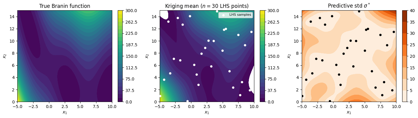
We now move to two dimensions. The Branin function is a standard benchmark in surrogate modeling and Bayesian optimization, defined on $[-5, 10] \times [0, 15]$:
\[f(x_1, x_2) = a\left(x_2 - b x_1^2 + cx_1 - r\right)^2 + s(1-t)\cos(x_1) + s\]with $a=1$, $b=5.1/(4\pi^2)$, $c=5/\pi$, $r=6$, $s=10$, $t=1/(8\pi)$. It has three global minima at roughly $(-\pi, 12.3)$, $(\pi, 2.3)$ and $(9.4, 2.5)$, making it a non-trivial test for a surrogate.
We sample $n = 30$ evaluation points using Latin Hypercube Sampling (LHS), a space-filling design that ensures uniform marginal coverage of the input domain with far fewer points than a regular grid. We then fit a GP with a Matérn $5/2$ kernel and hyperparameters optimized by marginal likelihood.
from scipy.stats import qmc
from sklearn.gaussian_process import GaussianProcessRegressor
from sklearn.gaussian_process.kernels import Matern, ConstantKernel
import warnings

def branin(x1, x2):
    a, b, c, r, s, t = 1, 5.1 / (4 * np.pi**2), 5 / np.pi, 6, 10, 1 / (8 * np.pi)
    return a * (x2 - b * x1**2 + c * x1 - r)**2 + s * (1 - t) * np.cos(x1) + s

# Latin Hypercube sampling
sampler = qmc.LatinHypercube(d=2, seed=0)
X_train_2d = qmc.scale(sampler.random(n=30), [-5, 0], [10, 15])
y_train_2d = branin(X_train_2d[:, 0], X_train_2d[:, 1])

# Fit GP with Matérn 5/2 kernel
kernel_2d = ConstantKernel() * Matern(nu=2.5)
with warnings.catch_warnings():
    warnings.simplefilter('ignore')
    gp = GaussianProcessRegressor(kernel=kernel_2d, n_restarts_optimizer=5, normalize_y=True)
    gp.fit(X_train_2d, y_train_2d)

print(f'Optimized kernel: {gp.kernel_}')

# Evaluate on a fine grid
x1g = np.linspace(-5, 10, 80)
x2g = np.linspace(0, 15, 80)
X1g, X2g = np.meshgrid(x1g, x2g)
X_grid = np.column_stack([X1g.ravel(), X2g.ravel()])

y_true_2d         = branin(X1g, X2g)
y_pred_2d, sig_2d = gp.predict(X_grid, return_std=True)
y_pred_2d = y_pred_2d.reshape(X1g.shape)
sig_2d    = sig_2d.reshape(X1g.shape)
Optimized kernel: 2.79**2 * Matern(length_scale=10.1, nu=2.5)
fig, axes = plt.subplots(1, 3, figsize=(14, 4))
levels = np.linspace(0, 300, 25)

c0 = axes[0].contourf(X1g, X2g, y_true_2d, levels=levels, cmap='viridis')
axes[0].set_title('True Branin function')
fig.colorbar(c0, ax=axes[0])

c1 = axes[1].contourf(X1g, X2g, y_pred_2d, levels=levels, cmap='viridis')
axes[1].scatter(X_train_2d[:, 0], X_train_2d[:, 1], c='white', s=20, zorder=5, label='LHS samples')
axes[1].set_title('Kriging mean ($n = 30$ LHS points)')
axes[1].legend(loc='upper right', fontsize=8)
fig.colorbar(c1, ax=axes[1])

c2 = axes[2].contourf(X1g, X2g, sig_2d, cmap='Oranges')
axes[2].scatter(X_train_2d[:, 0], X_train_2d[:, 1], c='k', s=20, zorder=5)
axes[2].set_title('Predictive std $\\sigma^*$')
fig.colorbar(c2, ax=axes[2])

for ax in axes:
    ax.set_xlabel('$x_1$')
    ax.set_ylabel('$x_2$')

plt.tight_layout()
plt.show()
So, why do we use kriging? The defining property of kriging is that it is the Best Linear Unbiased Estimator (BLUE): among all linear predictors that are unbiased on average, it minimizes the mean squared prediction error. This is not a coincidence of design — it follows from modeling the spatial covariance structure of the field. The prediction weights are not fixed by a geometric formula but are derived from the data’s own correlation.
Two further properties set kriging apart from simpler methods:
- Exact interpolation: in the noise-free case, predictions pass exactly through the observed values, and the predictive uncertainty collapses to zero at training points.
- Calibrated uncertainty: the predictive variance is large where data is sparse and small where data is dense, providing a principled map of where the estimate should not be trusted.
When kriging was developed, the competing methods for spatial interpolation shared a common weakness: their prediction weights were fixed by a geometric formula, not adapted to the structure of the data.
- Nearest neighbor (Voronoi/Thiessen polygons): assign each unsampled point the value of its closest observation. Exact at data points but produces step discontinuities at Voronoi boundaries and conveys no uncertainty.
- Inverse Distance Weighting (IDW): predict as a weighted average $\hat{f}(\mathbf{x}^\star) = \sum_i w_i y_i$ with $w_i \propto 1/d_i^p$, where $d_i$ is the distance to observation $i$ and $p$ is a user-chosen exponent (typically 2). Still common in GIS tools today, but the exponent is ad hoc, and a cluster of redundant nearby points is up-weighted the same as a single informative one — kriging avoids this by accounting for correlation between observations.
- Polynomial trend surfaces: fit a global low-degree polynomial by least squares. Captures large-scale spatial drift but cannot represent local variation, and carries no spatial structure in the residuals.
- Moving averages: compute a local weighted average within a search radius. Similar in spirit to IDW, with the same ad hoc weight structure.
Kriging’s key insight was to make the weights optimal by adapting them to the empirical covariance structure of the field, quantified by the variogram $\gamma(h) = \frac{1}{2}\operatorname{Var}[f(\mathbf{x}+h) - f(\mathbf{x})]$. This gave it the BLUE property that none of the above methods possess.
Kriging remains the method of choice for small-to-medium datasets (up to a few thousand points) where calibrated uncertainty is essential. Its main limitation is computational: solving the linear system $[K + \sigma_n^2 I]^{-1}\mathbf{y}$ costs $O(n^3)$ time and $O(n^2)$ memory, which becomes prohibitive as $n$ grows. Several approaches address this, or target different trade-offs entirely:
- Radial Basis Function (RBF) interpolation: mathematically nearly identical to kriging — both are kernel methods sharing the same prediction formula — but without the probabilistic framework, so there is no uncertainty estimate. Common in mesh-free numerical methods and computer graphics.
- Sparse / approximate GPs: replace the full $n \times n$ covariance system with a low-rank approximation using $m \ll n$ inducing points (methods: FITC, VFE, SVGP). Complexity drops to $O(nm^2)$, making GP regression practical for millions of observations. Libraries such as GPyTorch and GPflux implement these efficiently on GPU.
- Random forests and gradient boosting (XGBoost, LightGBM): excel on high-dimensional, mixed-type tabular data and require little tuning. Uncertainty is available but approximate (quantile regression, conformal prediction). Unlike kriging, they do not interpolate exactly and their predictions outside the training range revert to the empirical mean.
- Neural networks: scale to arbitrarily large datasets and can learn complex representations directly from raw inputs. Uncertainty requires extra effort (MC Dropout, deep ensembles, Bayesian NNs). Deep kernel learning combines a neural network feature extractor with a GP readout, capturing the representational power of deep learning with kriging-style uncertainty.
- Neural Processes: a meta-learning framework that amortizes GP-style inference into a neural network, enabling fast predictions for new observation sets without solving a linear system at test time.
Kriging is the natural starting point when the dataset is small (up to a few thousand points), the inputs are continuous and low-dimensional, and a reliable uncertainty estimate is required — as in surrogate modeling for expensive simulations, spatial mapping in geosciences, or as the probabilistic model inside a Bayesian optimization loop. For larger datasets or high-dimensional inputs, sparse GP approximations or deep learning methods are more practical, though they typically sacrifice some of the theoretical elegance and calibration guarantees that kriging provides.
To conclude, kriging is more than an interpolation formula — it is a fully probabilistic model that provides both a prediction and a calibrated uncertainty estimate. Its key ingredients are:
- A Gaussian process prior over functions, specified entirely by a covariance kernel.
- A covariance kernel (e.g. the Matérn family) that encodes smoothness assumptions via $\nu$ and controls the correlation range via the length scale $\ell$.
- Closed-form Bayesian updating: conditioning on data yields a tractable Gaussian predictive distribution with mean $\mu^\star$ and variance ${\sigma^\star}^2$ given by simple linear-algebra expressions.
- Hyperparameter optimization via marginal likelihood maximization, which balances data fit against model complexity.
The uncertainty estimate $\sigma^\star$ is large where data is sparse and collapses to zero at training points in the noise-free case. This property is exploited directly in Bayesian optimization, where acquisition functions such as Expected Improvement use both $\mu^\star$ and $\sigma^\star$ to balance exploitation and exploration.