Over the last two years some very interesting research has emerged that illustrates a fascinating connection between Deep Neural Nets and differential equations. In the previous post we have seen the applications to ordinary differential equations (ODEs); here we focus on partial differentil equations (PDEs).
Here, we use PINNs to approximate the solution of the one-dimensional PDE
\[\mathcal{N} (x, u(x)) = f(x, u(x)) \quad x \in \Omega \subset \mathbb{R}\]where $\mathcal{N}$ is a possibly nonlinear operator that depends on $x$, $u(x)$, and its derivatives $u’(x)$ and $u’‘(x)$. We focus on parabolic PDEs, and we assume that the problem above, completed by the appropriate boundary conditions, admits a unique solution. Our aim is to find an approximation $\hat{u}(x)$ to the true solution $u(x)$, that we suppose too difficult or impossible to compute analytically.
The fundamental difference compared to traditional approaches to solve PDEs is that PINNs calculate differential operators on graphs using automatic differentiation, while traditional approaches are based on numerical schemes. The basic formulation that we cover here does not require labeled data for training, and is unsupervised – they only require the evaluation of the residual function. There are indeed two networks: an approximation network and a residual network. The approximation network defines out approximation $\hat{u}(x)$ and depends on some trainable parameters; the residual network is used to compute, at a given point $x_i$, the $i$-th residual
\[R_i = \mathcal{N}(x_i, \hat{u}(x_i)) - f(x_i, \hat{u}(x_i)).\]The residuals for all the $M$ points $x_i, i = 1, \ldots, M$ are computed; their average define the loss function we want to minimize. The residual network is not trained and its only function is to feed the problem we want to solve to the optimizer. The distribution of the $M$ points in the domain $\Omega$ is important for the good convergence. Typically, one use a uniform distribution on simple domains, or pseudo- or quasi-random numbers.
Once a PINN is trained, the inference step provides in output the solution of the governing equation at the position specified by the input. PINNs are gridless methods because they do not require a grid. They borrow concepts from Newton-Krylov solvers (they aim to minimize the residual function), from finite element methods (they use basis functions) and Monte Carlo and Quasi-Monte Carlo method (to determine the points where to evaluate the residuals).
The literature on PINNs has grown substantially since their introduction. The main articles are:
- Physics Informed Deep Learning (Part I): Data-driven Solutions of Nonlinear Partial Differential Equations and Physics Informed Deep Learning (Part II): Data-driven Discovery of Nonlinear Partial Differential Equations, by Raisse, Perdikaris and Karniadakis, Nov 2017, introduce PINNS and demonstrates the concept by showing how to solve several classical PDEs;
- Physics-Informed Generative Adversarial Networks for Stochastic Differential Equations, by Yang, Zhang, and Karniadakis, addresses the problem of stochastic differential equations but uses a generative adversarial neural network;
- Highly-scalable, physics-informed GANs for learning solutions of stochastic PDEs, by Yang, Treichler, Kurth, Fischer, Barajas-Solano, Romero, Churavy, Tartakovsky, Houston, Prabhat, and Karniadakis, is the large study that applies the GAN PINNs techniques to the large scale problem of as uncertainty quantification of the models of subsurface flow at the Hanford nuclear site;
- On the Convergence and Generalization of Physics Informed Neural Networks, by Shin, Darbon and Karniadakis, is the theoretical proof that the PINNs approach really works.
We will only scratch the surface with a very simple problem – the one-dimensional Laplacian
\[- \Delta u(x) = f(x), \quad x \in (0, 1),\]with zero boundary conditions, $u(0) = 0$, $u(1) = 0$. The right-hand side is defined such that the solution reads
\[u(x) = \sin(\kappa \pi x),\]where $\kappa \in \mathbb{N}^+$ is a parameter that controls the smoothness of the solution and can be seen as a frequency. We introduce it to verify experimentally an important result is presented in Frequency Principle: Fourier Analysis Sheds Light on Deep Neural NetworkS, by Xu, Zhang, Luo, Xiao, and Ma. This result is called the Frequency principle (or F-principle) and shows that neural networks tend to fit target functions from low to high frequencies. This F-principle is opposite to the behavior of most conventional iterative solvers, which tend to converge faster for high frequencies and slowly for slow ones. We will see that, even for our simple problem, the higher the value for $\kappa$ the slower the convergence.
As always, we start with a few imports.
import matplotlib.pylab as plt
import numpy as np
import torch
torch.set_default_dtype(torch.float32)
from torch import nn
from torch.autograd import grad
The Model class defines our approximation $\hat{u}(x)$. The activation function must be at least twice differentiable, so we can’t use ReLU. We use a V-shaped network with four layers, with increasing number of nodes, however we note that for this simple problem the network structure is not too important.
Generally, PINNs are under-fitted: the network is not complex enough to accurately capture the relationship between the input variables at the collocation points and the solution. Therefore, they do not benefit from techniques developed for over-fitted networks, such as drop-out, which we don’t use.
class Model(nn.Module):
    def __init__(self):
        super(Model, self).__init__()
        self.layer1  = nn.Linear(1, 20)
        self.layer2  = nn.Linear(20, 40)
        self.layer3  = nn.Linear(40, 80)
        self.layer4  = nn.Linear(80, 1)
        self.activation  = nn.Tanh()
        for m in self.modules():
            if isinstance(m, nn.Linear):
                nn.init.normal_(m.weight, mean=0, std=0.1)

    def forward(self, x):
        x = self.activation(self.layer1(x))
        x = self.activation(self.layer2(x))
        x = self.activation(self.layer3(x))
        x = self.layer4(x)
        return x
def flat(x):
    m = x.shape[0]
    return [x[i] for i in range(m)]
π = np.pi
def exact_solution(x, κ):
    return torch.sin(κ * π * x)
This is the definition of our problem, and the only place where the equations come into play. The grad function computes the first and second derivative of our approximation $\hat{u}(x)$; this is combined with the right-hand side and returned to the optimizer.
def equation(model, x, κ):
    u = model(x)
    u_x = grad(flat(u), x, create_graph=True, allow_unused=True)[0]
    u_xx = grad(flat(u_x), x, create_graph=True, allow_unused=True)[0]
    lhs = -u_xx
    rhs = κ**2 * π**2 * torch.sin(κ * π * x)
    return lhs, rhs
x_boundary = torch.tensor([[0.0], [1.0]])
bc = torch.FloatTensor([[0.0], [0.0]])
The loss function uses a hyperparameter $\lambda$ to balance the loss of interior nodes with that of boundary nodes, and follows the definition reported in Estimates on the generalization error of Physics Informed Neural Networks for approximating PDEs by Siddhartha Mishra and Roberto Molinaro. As in this simple problem the boundary is only composed by two nodes, we use $\lambda=1$.
num_points = 128
num_epochs = 5_000
λ = 1.0
x_sample = torch.linspace(0, 1, 10_000).unsqueeze(-1)
u_exact_sample = exact_solution(x_sample.flatten(), κ).numpy()
def solve(model, num_points, num_epochs, lr, κ, λ, print_every=None):
    loss_fn = nn.MSELoss()
    optimizer = torch.optim.Adam(model.parameters(), lr=lr)

    history = []
    errors = []

    for epoch in range(num_epochs):
        optimizer.zero_grad()
        u_boundary = model(x_boundary)
        x = torch.rand((num_points, 1), requires_grad=True, dtype=torch.float32)
        lhs, rhs = equation(model, x, κ)
        # scale the internal residual to have similar numbers for any values of κ
        loss = (loss_fn(lhs, rhs) + λ * loss_fn(u_boundary, bc)) / (κ**2)
        loss.backward()
        optimizer.step()
        history.append(loss.detach().numpy())
        if print_every is not None and (epoch + 1) % print_every == 0:
            print(epoch + 1, history[-1])
        with torch.no_grad():
            u_approx_sample = model(x_sample).detach().flatten().numpy()
            errors.append(abs(u_approx_sample - u_exact_sample).mean())

    return history, errors
We use $\kappa={2, 4, 8}$. After a small hyperparameter optimization, the learning rate is set to 0.001 for all values of $\kappa$.
model_2 = Model()
history_2, errors_2 = solve(model_2, num_points, num_epochs, lr=0.001, κ=2, λ=λ)
model_4 = Model()
history_4, errors_4 = solve(model_4, num_points, num_epochs, lr=0.001, κ=4, λ=λ)
model_8 = Model()
history_8, errors_8 = solve(model_8, num_points, num_epochs, lr=0.001, κ=8, λ=λ)
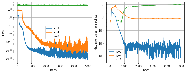
It is not straightforward to compare the results with different $\kappa$ values (because of the $\pi^2 \kappa^2$ scaling in the right-hand side, which we try to remove), however the graphs below show some interesting phenomena. Looking at the loss function, we see a small plateau at the beginning, which gets longer as $\kappa$ grows. For $\kappa=1$, it seems that about one thousand iterations suffice (after that, the optimizer stagnates); for $\kappa=2$, it takes about two thousand iterations to stagnate, while $\kappa=8$ hasn’t converged at all, as we will see below.
fig, (ax0, ax1) = plt.subplots(figsize=(10, 4), ncols=2)
for history, κ in [(history_2, 2), (history_4, 4), (history_8, 8)]:
    ax0.semilogy(history, label=f'κ={κ}')
ax0.grid()
ax0.set_xlabel('Epoch')
ax0.set_ylabel('Loss')
ax0.legend()
for errors, κ in [(errors_2, 2), (errors_4, 4), (errors_8, 8)]:
    ax1.semilogy(errors, label=f'κ={κ}')
ax1.grid()
ax1.set_xlabel('Epoch')
ax1.set_ylabel('Max error on sample points')
ax1.legend()
fig.tight_layout()
def plot(model, κ):
    fig, (ax0, ax1) = plt.subplots(figsize=(10, 4), ncols=2)
    x_unif = torch.linspace(0, 1, 201).unsqueeze(-1)
    y_approx = model(x_unif).detach().numpy()
    ax0.plot(x_unif.numpy(), y_approx, label=r'$\hat{u}(x), \kappa=' + str(κ) + '$')
    y_exact = exact_solution(x_unif, κ).numpy()
    ax0.plot(x_unif.numpy(), y_exact, label=r'$u(x), \kappa=' + str(κ) + '$')
    ax1.plot(x_unif.numpy(), y_approx - y_exact, label=f'κ={κ}')
    ax0.set_xlabel('x')
    ax0.legend(loc='upper right')
    ax0.set_title('Functions')
    ax1.set_xlabel('x')
    ax1.set_ylabel(r'$\hat{u}(x) - u(x)$')
    ax1.set_title('Error')
    ax1.legend()
    fig.tight_layout()
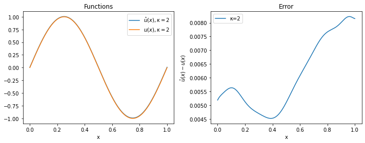
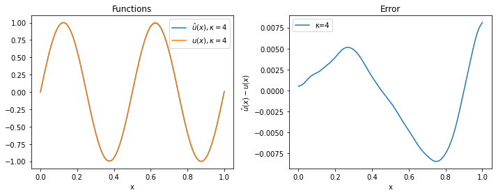
For $\kappa=2$ and $\kappa=4$, the approximation is quite good, while for $\kappa=8$ the solver has clearly not managed to provide a reasonable solution (even if more iterations or a smaller learning rate would probably solve the problem).
plot(model_2, 2)
plot(model_4, 4)
plot(model_8, 8)
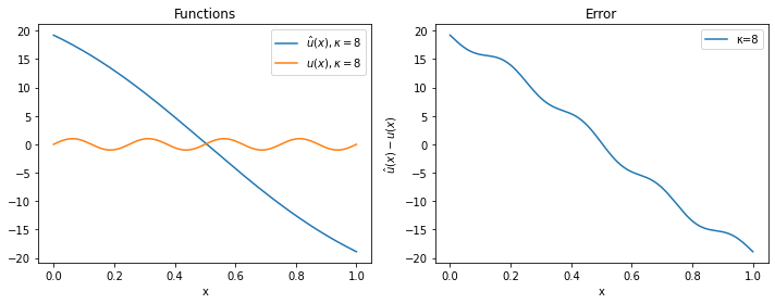
These results show that, because of the F-principle, PINNs converge quickly to the low frequencies of the solution; the convergence to the high frequencies is slow and requires many more epochs, as we have seen. Because of this, PINNs tend to be of limited usage when the application requires highly accurate solutions that contain high frequency modes. They will shine more with nonlinear problems and complex, high-dimensional domains, as we will show in following posts.