Our goal is to use a linear regression model, implemented in PyTorch, for thr boston housing dataset contained in the scikit-learn package. We start by loading the data, performing some basic data analysis and visualization, then finally building the PyTorch model and fitting it. Although linear models exist in scikit-learn (and are very easy to use for this example), we want to play with PyTorch on a simple yet interesting problem.
import matplotlib.pyplot as plt
import numpy as np
import pandas as pd
import seaborn as sns
from sklearn import datasets
from sklearn.metrics import mean_squared_error, r2_score
from sklearn.model_selection import train_test_split
As first step we load the dataset and print out the DESCR field.
boston = datasets.load_boston()
print(boston['DESCR'])
.. _boston_dataset:

Boston house prices dataset
---------------------------

**Data Set Characteristics:**

    :Number of Instances: 506

    :Number of Attributes: 13 numeric/categorical predictive. Median Value (attribute 14) is usually the target.

    :Attribute Information (in order):
        - CRIM     per capita crime rate by town
        - ZN       proportion of residential land zoned for lots over 25,000 sq.ft.
        - INDUS    proportion of non-retail business acres per town
        - CHAS     Charles River dummy variable (= 1 if tract bounds river; 0 otherwise)
        - NOX      nitric oxides concentration (parts per 10 million)
        - RM       average number of rooms per dwelling
        - AGE      proportion of owner-occupied units built prior to 1940
        - DIS      weighted distances to five Boston employment centres
        - RAD      index of accessibility to radial highways
        - TAX      full-value property-tax rate per $10,000
        - PTRATIO  pupil-teacher ratio by town
        - B        1000(Bk - 0.63)^2 where Bk is the proportion of blacks by town
        - LSTAT    % lower status of the population
        - MEDV     Median value of owner-occupied homes in $1000's

    :Missing Attribute Values: None

    :Creator: Harrison, D. and Rubinfeld, D.L.

This is a copy of UCI ML housing dataset.
https://archive.ics.uci.edu/ml/machine-learning-databases/housing/


This dataset was taken from the StatLib library which is maintained at Carnegie Mellon University.

The Boston house-price data of Harrison, D. and Rubinfeld, D.L. 'Hedonic
prices and the demand for clean air', J. Environ. Economics & Management,
vol.5, 81-102, 1978.   Used in Belsley, Kuh & Welsch, 'Regression diagnostics
...', Wiley, 1980.   N.B. Various transformations are used in the table on
pages 244-261 of the latter.

The Boston house-price data has been used in many machine learning papers that address regression
problems.

.. topic:: References

   - Belsley, Kuh & Welsch, 'Regression diagnostics: Identifying Influential Data and Sources of Collinearity', Wiley, 1980. 244-261.
   - Quinlan,R. (1993). Combining Instance-Based and Model-Based Learning. In Proceedings on the Tenth International Conference of Machine Learning, 236-243, University of Massachusetts, Amherst. Morgan Kaufmann.
num_features = len(boston['feature_names'])
num_instances = len(boston['data'])
print(f"The dataset has {num_features} features, whose names are: {', '.join(boston['feature_names'])}")
print(f"There are {num_instances} instances")
The dataset has 13 features, whose names are: CRIM, ZN, INDUS, CHAS, NOX, RM, AGE, DIS, RAD, TAX, PTRATIO, B, LSTAT
There are 506 instances
An easy way to get a sense of what the dataset contains is to convert it into a Pandas DataFrame and use the describe() method.
df = pd.DataFrame(boston.data, columns=boston['feature_names'])
df.describe().round(2)
| CRIM | ZN | INDUS | CHAS | NOX | RM | AGE | DIS | RAD | TAX | PTRATIO | B | LSTAT | |
|---|---|---|---|---|---|---|---|---|---|---|---|---|---|
| count | 506.00 | 506.00 | 506.00 | 506.00 | 506.00 | 506.00 | 506.00 | 506.00 | 506.00 | 506.00 | 506.00 | 506.00 | 506.00 |
| mean | 3.61 | 11.36 | 11.14 | 0.07 | 0.55 | 6.28 | 68.57 | 3.80 | 9.55 | 408.24 | 18.46 | 356.67 | 12.65 |
| std | 8.60 | 23.32 | 6.86 | 0.25 | 0.12 | 0.70 | 28.15 | 2.11 | 8.71 | 168.54 | 2.16 | 91.29 | 7.14 |
| min | 0.01 | 0.00 | 0.46 | 0.00 | 0.38 | 3.56 | 2.90 | 1.13 | 1.00 | 187.00 | 12.60 | 0.32 | 1.73 |
| 25% | 0.08 | 0.00 | 5.19 | 0.00 | 0.45 | 5.89 | 45.02 | 2.10 | 4.00 | 279.00 | 17.40 | 375.38 | 6.95 |
| 50% | 0.26 | 0.00 | 9.69 | 0.00 | 0.54 | 6.21 | 77.50 | 3.21 | 5.00 | 330.00 | 19.05 | 391.44 | 11.36 |
| 75% | 3.68 | 12.50 | 18.10 | 0.00 | 0.62 | 6.62 | 94.07 | 5.19 | 24.00 | 666.00 | 20.20 | 396.22 | 16.96 |
| max | 88.98 | 100.00 | 27.74 | 1.00 | 0.87 | 8.78 | 100.00 | 12.13 | 24.00 | 711.00 | 22.00 | 396.90 | 37.97 |
It is also convenient to check that we have no nan’s in the dataset, as they would cause problems in the model calibration.
df.isnull().any()
CRIM       False
ZN         False
INDUS      False
CHAS       False
NOX        False
RM         False
AGE        False
DIS        False
RAD        False
TAX        False
PTRATIO    False
B          False
LSTAT      False
dtype: bool
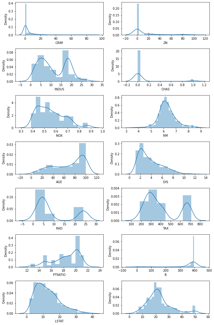
Whenever possible it is convenient to explore the data visually, for example with density plots, as done below.
import warnings
warnings.simplefilter(action='ignore', category=FutureWarning)  # some scipy issues

fig, axes = plt.subplots(nrows=7, ncols=2, figsize=(10, 15))
sns.distplot(df['CRIM'], ax=axes[0, 0])
sns.distplot(df['ZN'], ax=axes[0, 1])
sns.distplot(df['INDUS'], ax=axes[1, 0])
sns.distplot(df['CHAS'], ax=axes[1, 1])
sns.distplot(df['NOX'], ax=axes[2, 0])
sns.distplot(df['RM'], ax=axes[2, 1])
sns.distplot(df['AGE'], ax=axes[3, 0])
sns.distplot(df['DIS'], ax=axes[3, 1])
sns.distplot(df['RAD'], ax=axes[4, 0])
sns.distplot(df['TAX'], ax=axes[4, 1])
sns.distplot(df['PTRATIO'], ax=axes[5, 0])
sns.distplot(df['B'], ax=axes[5, 1])
sns.distplot(df['LSTAT'], ax=axes[6, 0])
sns.distplot(boston.target, ax=axes[6, 1])
plt.tight_layout()
It is also useful to plot the dependency on the individual features. This command takes several seconds if ran on the full dataset, and results in an image with too many graphs; instead, we select a few columns that seem important from the description above. However, no clear relationship emerges from this graph among those variables.
sns.pairplot(df[['AGE', 'RAD', 'RM', 'TAX', 'DIS']])
<seaborn.axisgrid.PairGrid at 0x1404b3531f0>

At this point we can build the linear regression model. As customary, we split the dataset into a training set, composed the 80% of the data, and a test set, with the remaining 20% of the data.
X = boston.data
y = boston.target
X_train, X_test, y_train, y_test = train_test_split(X, y, test_size=0.2)
print(f"Selected {len(X_train)} instances for training the model and {len(X_test)} to test it.")
Selected 404 instances for training the model and 102 to test it.
As a final preprocessing step, we rescale the data. This is not stricly necessary with linear regression, yet it is a good habit and will give more meaning to the coefficients of the linear model.
from sklearn.preprocessing import StandardScaler
scaler = StandardScaler()
X_train_scaled = scaler.fit_transform(X_train)
X_test_scaled = scaler.fit_transform(X_test)
As scikit-learn offers a linear regression model, we build it and display the coefficients. We will use this model to check out PyTorch implementation.
from sklearn.linear_model import LinearRegression
sk_model = LinearRegression()
sk_model.fit(X_train_scaled, y_train)
R2 = sk_model.score(X_test_scaled, y_test)
print(f"R2 score = {R2:.3f}")
R2 score = 0.679
print("\ty_hat = ")
for name, coeff in zip(boston['feature_names'], sk_model.coef_):
    print(f"\t{coeff:+6.2f} x {name}")
print(f"\t{sk_model.intercept_:+6.2f}")
	y_hat =
	 -0.98 x CRIM
	 +1.23 x ZN
	 +0.01 x INDUS
	 +0.80 x CHAS
	 -2.23 x NOX
	 +3.05 x RM
	 +0.05 x AGE
	 -3.31 x DIS
	 +2.70 x RAD
	 -2.17 x TAX
	 -1.85 x PTRATIO
	 +0.79 x B
	 -3.36 x LSTAT
	+22.92
Let’s turn now our attention to the PyTorch implementation. Although in real life we would not use an iterative solver for this task, here we do and run 5’000 iterations, after which the coefficients are very close to the ones provided by scikit-learn.
import torch
import torch.nn as nn
class LR(nn.Module):
    def __init__(self, input_size, output_size):
        super().__init__()
        self.linear = nn.Linear(input_size, output_size, bias=True)

    def forward(self, x):
        return self.linear(x)
model = LR(X_test_scaled.shape[1], 1)
criterion = nn.MSELoss()
optimizer = torch.optim.SGD(model.parameters(), lr=0.01)

num_epochs = 5_000
losses = []
for epoch in range(num_epochs):
    optimizer.zero_grad()
    x = torch.tensor(X_train_scaled, dtype=torch.float32)
    y = torch.tensor(y_train, dtype=torch.float32).reshape([404, 1])
    y_hat = model.forward(x)
    loss = criterion(y_hat, y)
    if (epoch + 1) % 1_000 == 0:
        print(f"epoch: {epoch + 1}, loss: {loss.item()}")
    loss.backward()
    optimizer.step()
epoch: 1000, loss: 22.501567840576172
epoch: 2000, loss: 22.43768310546875
epoch: 3000, loss: 22.4332218170166
epoch: 4000, loss: 22.432891845703125
epoch: 5000, loss: 22.432870864868164
w = model.state_dict()['linear.weight'][0]
b = model.state_dict()['linear.bias'][0]

print("\ty_hat = ")
for name, coeff in zip(boston['feature_names'], w):
    print(f"\t{coeff:+6.2f} x {name}")
print(f"\t{b:+6.2f}")
	y_hat =
	 -0.98 x CRIM
	 +1.23 x ZN
	 +0.01 x INDUS
	 +0.80 x CHAS
	 -2.23 x NOX
	 +3.05 x RM
	 +0.05 x AGE
	 -3.31 x DIS
	 +2.69 x RAD
	 -2.17 x TAX
	 -1.85 x PTRATIO
	 +0.79 x B
	 -3.36 x LSTAT
	+22.92
In the optimizer loop above, we have used the dataset in its entirety because of the small size. In general, however, we need to operate on batches of smaller sizes, say 64 or 256, and we also want to test the performances of the model on the validation dataset as we go through the epochs. It is easy to do so in PyTorch using the Dataset class: what we need to implement is the __len__() method, returning the length of the dataset, and the __getitem__() method,
which returns, in PyTorch format, the features and values. Another PyTorch class, DataLoader, will take care of loading the data from our Dataset-derived class, shuffle them if needed, and return batched of the requested size. It is easy to load images from files or augment the data for classification tasks, for example by using an image and its reflected version in case this makes sense for the problem at hand.
class Dataset(torch.utils.data.Dataset):
    def __init__(self, X, y):
        # constructor, we store X (features) and y (values to predict)
        assert len(X) == len(y)
        self.X = X
        self.y = y

    def __len__(self):
        # lenght of the dataset
        return len(self.X)

    def __getitem__(self, index):
        # returns the index-th element
        X = torch.tensor(self.X[index], dtype=torch.float32)
        y = torch.tensor(self.y[index], dtype=torch.float32).reshape(1)
        return X, y
To obtain the same results we got above, we need to use a batch size large enough to contain the entire dataset in one batch. Alternatively, we can try smaller batch sizes and iterate longer. The coefficients returned by the model can be printed out with the same code used before.
criterion = nn.MSELoss()
optimizer = torch.optim.SGD(model.parameters(), lr=0.01)

params = {'batch_size': 512, 'shuffle': True}
max_epochs = 5_000

dataset_train = Dataset(X_train_scaled, y_train)
generator_training = torch.utils.data.DataLoader(dataset_train, **params)

dataset_validation = Dataset(X_test_scaled, y_test)
generator_validation = torch.utils.data.DataLoader(dataset_validation, **params)

device = 'cpu'  # or 'cuda' if available
for epoch in range(max_epochs):
    # Training
    total_training_loss = 0.0
    for X_batch, y_batch in generator_training:
        optimizer.zero_grad()
        X_batch, y_batch = X_batch.to(device), y_batch.to(device)
        y_batch_pred = model.forward(X_batch)
        loss = criterion(y_batch_pred, y_batch)
        total_training_loss += loss.item()
        loss.backward()
        optimizer.step()
    # Validation
    with torch.set_grad_enabled(False):
        total_validation_loss = 0.0
        for X_batch, y_batch in generator_validation:
            X_batch, y_batch = X_batch.to(device), y_batch.to(device)
            X_batch, y_batch = X_batch.to(device), y_batch.to(device)
            y_batch_pred = model.forward(X_batch)
            loss = criterion(y_batch_pred, y_batch)
            total_validation_loss += loss.item()
    if (epoch + 1) % 1_000 == 0:
        print(f"epoch: {epoch + 1}, training loss: {total_training_loss}, val loss: {total_validation_loss}")
epoch: 1000, training loss: 22.43286895751953, val loss: 23.72454261779785
epoch: 2000, training loss: 22.43286895751953, val loss: 23.724536895751953
epoch: 3000, training loss: 22.43286895751953, val loss: 23.72454071044922
epoch: 4000, training loss: 22.43286895751953, val loss: 23.724536895751953
epoch: 5000, training loss: 22.43286895751953, val loss: 23.72454261779785