In this article we start exploring policy methods, that is methods that aim to define the policy fuction $\pi(S_t)$. The policy function is the entity that tells us what to do in every state $S_t$. For methods based on the $Q-$values, the policy is derived indirectly from all the $Q-$values for a given state; hwre instead we aim to define the policy directly. There are several reasons why this may be a good choice. First, in environments with lots of actions the $Q-$value function has several entries. At the limit of infinite actions, that is with continuous action spaces, the $Q-$values approach won’t work, while the policy methods will. Second, policy methods can potentially learn the optimal policy even if this is stochastic. Of course we’ll use neural networks to approximate the policy, however simpler methods could be used as well, see Section 13.1 of the Sutton and Barto book.
For discrete action spaces a common approach is to let the neural network return the probabilities of the actions; a multinomial distribution is then used to produce the selected action. Such representation of actions as probabilities has the advantage of being smooth: if we change our network weights a bit, the output of the network (that is, the probability distribution) will generally change a bit as well.
Here we implement the REINFORCE method. The method was proposed by R. Williams in 1992 in the paper Simple Statistical Gradient-Following Algorithms for Connectionist Reinforcement Learning, Machine Learning, 8, 229-256. The paper says that the name is an acronym for “REward Increment = Nonnegative Factor x Offset Reinforcement x Characteristic Eligibility”, which is the equation described at page 234. The notation of the paper is slightly different from what is generally used today, so to understand the method it’s easier to read the Sutton and Barto book.
The code is taken from the official PyTorch example, then changed a bit. The implementation is quite simple and almost all of the logic is contained in the finish_episode() method. The method is the basic one without baselines.
import gym
import numpy as np
from itertools import count
from collections import deque
import matplotlib.pylab as plt
import torch
import torch.nn as nn
import torch.nn.functional as F
import torch.optim as optim
from torch.distributions import Categorical
device = torch.device("cuda:0" if torch.cuda.is_available() else "cpu")
We will use the Lunar Lander environment as it can be solved with this method.
ENV_NAME = 'LunarLander-v2'
GAMMA = 0.99
SEED = 543
LOG_INTERVAL = 100
env = gym.make(ENV_NAME)
num_observations = env.observation_space.shape[0]
num_actions = env.action_space.n
print(f"Observation space size: {num_observations}, # actions: {num_actions}")
Observation space size: 8, # actions: 4
We define the main class, which contains the (simple) neural network that is used to approximate the policy. The network won’t learn unless the numbers it operates on are reasonably scaled; in our case we aim to scale the sum of the returns to be normal. As we don’t know the mean and the standard deviation, we estimate it by the values we get during the training phase. The training logic is contained in the finish_episode() method, which uses the gradient
\(\nabla J(\theta) = E_\pi
\left[
G_t \nabla \ln \pi(A_t | S_t, \theta)
\right],\)
see page 327 of the Sutton and Barto book, second edition. The expression in the expectation can be computed on each time step once an episode is finished and says that the increment is the product of the a return $G_t$ and a vector, the gradient of the probability of taking the action actually taken divided by the probability of taking that action.
Note that there is no explicit exploration: since the action is selected using a multinomial probability distribution, the exploration is performed automatically.
class Policy(nn.Module):
    def __init__(self):
        super(Policy, self).__init__()
        self.affine1 = nn.Linear(num_observations, 64)
        self.dropout = nn.Dropout(p=0.6)
        self.affine2 = nn.Linear(64, num_actions)

        self.saved_log_probs = []
        self.rewards = []

        self.eps = np.finfo(np.float32).eps.item()

        # to estimate the mean and std dev of the returns, such that
        # the neural network only works on normalized numbers
        self.num_returns = 0
        self.sum_returns = 0.0
        self.sum_returns_squared = 0.0

    def forward(self, x):
        x = self.affine1(x)
        x = self.dropout(x)
        x = F.relu(x)
        action_scores = self.affine2(x)
        return F.softmax(action_scores, dim=1)

    def select_action(self, state):
        state = torch.from_numpy(state).float().unsqueeze(0)
        probs = self(state)
        m = Categorical(probs)
        action = m.sample()
        self.saved_log_probs.append(m.log_prob(action))
        return action.item()

    def finish_episode(self):
        G = 0
        policy_loss = []
        returns = []
        for r in self.rewards[::-1]:
            G = r + GAMMA * G
            returns.insert(0, G)
            self.num_returns += 1
            self.sum_returns += G
            self.sum_returns_squared += G**2
        returns = torch.tensor(returns)
        returns_mean = self.sum_returns / self.num_returns
        returns_std_dev = np.sqrt(self.sum_returns_squared / self.num_returns - returns_mean**2)
        returns = (returns - returns_mean) / (returns_std_dev + self.eps)

        for log_prob, R in zip(self.saved_log_probs, returns):
            policy_loss.append(-log_prob * R)
        optimizer.zero_grad()
        policy_loss = torch.cat(policy_loss).sum()
        policy_loss.backward()
        optimizer.step()
        del self.rewards[:]
        del self.saved_log_probs[:]
REINFORCE, as other policy methods, is on-policy; fresh samples from the environment are required to proceed with the training. We can also note that we only access the neural network once, to get the probabilities of action, while methods like DQN requires two, one for the current state and the other for the next state in the Bellman update. It is also evident is that full episodes are needed – for complicated tasks which result in long episodes, this can be a severe limitation. A more serious problem is the large correlation between the samples. As we said, we generate a full episode and then we train. We can’t use a replay memory since we need the samples to be generated by the current policy; instead, often people use parallel environments and use their transitions as training data with less correlation.
env.seed(SEED)
_ = torch.manual_seed(SEED)

reinforce = Policy()
optimizer = optim.Adam(reinforce.parameters(), lr=1e-2)

running_rewards = deque(maxlen=100)
running_means = []
running_std_devs = []
episode_lengths = []
episode_rewards = []

for i_episode in range(1, 10_001):
    state, episode_reward = env.reset(), 0.0
    for t in range(1, 5_000):  # Don't infinite loop while learning
        action = reinforce.select_action(state)
        state, reward, done, _ = env.step(action)
        reinforce.rewards.append(reward)
        episode_reward += reward
        if done:
            break

    episode_lengths.append(t)
    episode_rewards.append(episode_reward)

    # update cumulative reward
    running_rewards.append(episode_reward)

    # perform backprop
    reinforce.finish_episode()

    mean = np.array(running_rewards).mean()
    std_dev = np.array(running_rewards).std()
    running_means.append(mean)
    running_std_devs.append(std_dev)

    # log results
    if i_episode % LOG_INTERVAL == 0:
        print(f"Episode {i_episode}\tRunning average reward: {mean:.2f}, std dev: {std_dev:.2f}")

    if mean > env.spec.reward_threshold:
        print(f"Solved! Running reward is now {mean:.2f} and the last episode runs to {t} time steps!")
        break
Episode 100	Running average reward: -174.67, std dev: 110.92
Episode 200	Running average reward: -128.64, std dev: 66.37
Episode 300	Running average reward: -111.89, std dev: 51.31
Episode 400	Running average reward: -104.08, std dev: 122.00
Episode 500	Running average reward: -68.92, std dev: 88.25
Episode 600	Running average reward: -20.49, std dev: 63.68
Episode 700	Running average reward: -30.84, std dev: 68.17
Episode 800	Running average reward: 2.51, std dev: 87.19
Episode 900	Running average reward: 46.44, std dev: 84.19
Episode 1000	Running average reward: 62.02, std dev: 125.79
Episode 1100	Running average reward: 86.62, std dev: 128.10
Episode 1200	Running average reward: 122.29, std dev: 156.24
Episode 1300	Running average reward: 187.94, std dev: 114.57
Episode 1400	Running average reward: 163.10, std dev: 122.77
Episode 1500	Running average reward: 185.22, std dev: 109.39
Episode 1600	Running average reward: 98.53, std dev: 116.95
Episode 1700	Running average reward: 108.87, std dev: 132.48
Episode 1800	Running average reward: 181.16, std dev: 108.07
Solved! Running reward is now 200.26 and the last episode runs to 269 time steps!
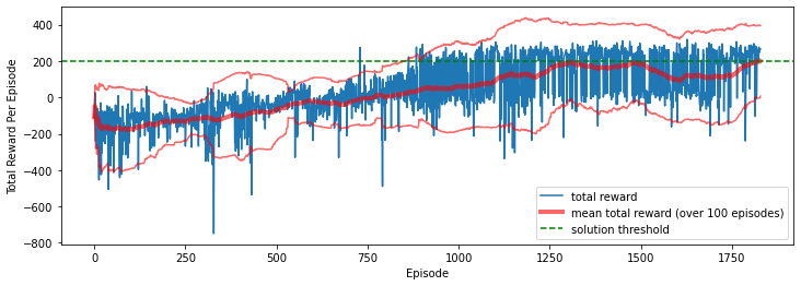
The method converges, albeit quite slowly and with a non-monotonic convergence. Possibly a different learning rate or more nodes in the neural network would have improved the results (using 128 hidden nodes leads to a convergence in 4,200 episodes while a smaller dropout rate results in a much worse convergence). There is still quite some variability in the results, as seen in the picture below which reports the total rewards per episode over the 1,800 episodes that it takes to solve the problem, as well as the mean and the standard deviation over the last 100 episodes. The confidence interval is reported: note that the distribution isn’t symmetric but rather skewed towards bad results. This is expected: on one side, it’s easier to make mistake than to do fantastic things by chance; on the other side, the maximum reward is limited. This means that our policy will be generally good, but in some cases it may fail completely.
plt.figure(figsize=(12, 4))
plt.plot(episode_rewards, label='total reward')
plt.plot(running_means - 1.96 * np.array(running_std_devs), color='red', alpha=0.6)
plt.plot(running_means, linewidth=4, color='red', alpha=0.6, label='mean total reward (over 100 episodes)')
plt.plot(running_means + 1.96 * np.array(running_std_devs), color='red', alpha=0.6)
plt.axhline(y=200, linestyle='dashed', color='green', label='solution threshold')
plt.legend(loc='lower right')
plt.xlabel('Episode')
plt.ylabel('Total Reward Per Episode');
state = env.reset()
video = [env.render(mode='rgb_array')]
done = False
total_reward = 0.0
while not done:
    action = reinforce.select_action(state)
    state, reward, done, _ = env.step(action)
    total_reward += reward
    video.append(env.render(mode='rgb_array'))
print(f"# steps: {len(video) - 1}, total reward: {total_reward:.2f}")
video = np.array(video)
# steps: 278, total reward: 261.08
from matplotlib import pyplot as plt
from matplotlib import animation
fig = plt.figure(figsize=(8, 8))
im = plt.imshow(video[0,:,:,:])
plt.axis('off')
plt.close() # this is required to not display the generated image

def init():
    im.set_data(video[0,:,:,:])

def animate(i):
    im.set_data(video[i,:,:,:])
    return im

anim = animation.FuncAnimation(fig, animate, init_func=init, frames=video.shape[0], interval=100)
anim.save('./lunar-lander-video.mp4')
As we said in the introduction we have used the basic REINFORCE without baselines. This isn’t used much on its own because the gradient update has large variance, rendering the training process unstable. The solution is to add a baseline, akin to the variance reduction approaches that are used in Monte Carlo procedures. This brings us to the so-called actor-critic methods, often referred to as advantage actor-critic methods. We will explore A2C methods in another article.