The Merton Jump Diffusion Model

In this article we study the Merton jump diffusion process, first proposed in 1976. The model can be seen as an extension of the Black-Scholes model with superimposed jumps. We suppose that at a jump the stock price is multiplied by a (random) value $J$, which we will need to model. We can write the process, in the $\mathbb{Q}$ measure as

\[\frac{dS(t)}{S(t^-)} = (r - q) dt + \sigma dW(t) + dJ,\]

where $r$ is the constant interest rate, $q$ the constant dividend, $\sigma$ the volatility of the diffusion part, while $dJ$ is the jump part. Since at a jump the spot process is discontinuous, we have used $S(t^-)$ to indicate the value of the spot process just before the jump, as for càdlàg processes. Financially, this means that we cannot hope to predict or manage in any way the jump as it happens suddenly.

The jump component is the compound Poisson process

\[J(t) = \sum_{j=1}^{N(t)} (Y_j - 1),\]

where $N(t)$ is a counting process satisfying $N(t) = \sup { n: \tau_n \le t }$ and each $\tau_h$ is a jump time, with $Y_j$ the corresponding jump size. The jumps are multiplicative: at $t= \tau_j$,

\[\begin{aligned} \frac{S(t) - S(t^-)}{S(t^-)} & = (Y_j - 1) \\ % S(t) - S(t^-) & = Y_j S(t^-) - S(t^-) \\ % S(t) & = Y_j S(t^-), \end{aligned}\]

where $S(t^-)$ is the value of the spot process just before the spot; the $Y_j$ are therefore positive multipliers of the spot.

We need to model $N(t)$ and the $Y_j$, which must be positive such that the price remains positive as well; let’s start from $N(t)$. In the Merton model, $N(t)$ is a Poisson counting process with intensity $\lambda > 0$. The probability that there are $n$ jumps in the interval $[0, t]$ is

\[\mathbb{P}[N(t) = n] = e^{-\lambda t} \frac{(\lambda t)^n}{n!}.\]

The interarrival times $\tau_{j+1}-\tau_j$ are independent and have a common exponential distribution,

\[\mathbb{P}[\tau_{j+1}-\tau_j \le t] = 1 - e^{-\lambda t}, \quad t \ge 0.\]

We also known that

\[\mathbb{E}[N(t)] = \lambda t.\]

If we further assume that the $Y_j$ are i.i.d. and independent of $N$ and $W$, we have a compound Poisson process, for which

\[\mathbb{E}[J(t)] = \lambda t \mathbb{E}[Y_j].\]

It is possible to find an analytic solution if we also assume the $Y_j$ to be lognormal with mean $\mu$ and variance $\delta^2$, that is $Y_j \sim \mathcal{LN}(\mu, \delta^2)$ and $\mathbb{E}[Y_j] = e^{\mu + \frac{1}{2}\delta^2}$. Therefore,

\[\mathbb{E}[J(t)] = \lambda t \left( e^{\mu + \frac{1}{2} \delta^2} - 1\right) = \lambda t m.\]

Overall, the parmeters are:

• $r$: the continuously compounded interest rate;
• $q$: the continuously compounded dividens;
• $\sigma$: the volatility of the diffusion part;
• $\lambda$: the jump intensity;
• $\mu$: the mean jump size (in logspot);
• $\delta^2$: the variance of the jump size (in logspot).

Because of the assumption on the jumps, $Y_j \sim \mathcal{LN}(\mu, \delta^2)$, we have

\[\mathbb{E}[Y_j - 1] = e^{a + \frac{1}{2}b^2} - 1 = m.\]

Conditional on $N(T) = n$, the spot distribution at $t=T$ is lognormal,

\[S(T) \sim \mathcal{N} \left( \log S_0 + \left( \mu - \frac{1}{2} \sigma^2 - \lambda m \right) T + an, \sigma^2 T + b^2 n \right),\]

so the value of an option is given by the Black-Scholes formula with a forward $F(T) = S_0 e^{(\mu - \frac{1}{2}\sigma^2 - \lambda m)T + a n}$ and variance $\sigma^2 T + b^2 n$, that is

\[e^{-r T} \left( F \Phi(d_+) - K \Phi(d_-) \right),\]

where $\Phi$ is the cumulative density function of the normal distribuion. From the definition of $m$ we easily obtain

\[\mu = \log(m + 1) - \frac{1}{2}\delta^2,\]

that is

\[F(T) = S_0 e^{(\mu - \frac{1}{2} \sigma^2 - \lambda m)T + n \log(m+1) - \frac{1}{2}\mu^2n},\]

which allows us to introduce a discount factor

\[r_n = r - \lambda m + n \log(1 + m) / T\]

and rewrite our solution as

\[e^{-r_n T} e^{-\lambda m T} \left[ e^{\log(1 + m)} \right]^n \left[ F \Phi(d_+) - K \Phi(d_-) \right].\]

Since the probability of $N(T) = n$ is given by $e^{-\lambda T} (\lambda T)^n / n!$, we get

\[\begin{aligned} e^{-r T} \mathbb{E}[(S(T) - K)^+] & = \sum_{n=0}^\infty e^{-\lambda T} \frac{(\lambda T)^n}{n!} e^{-\lambda m T} (1 + m)^n BS(S_0, K, T, r_n, \mu, \sigma_n) \\ % & = \sum_{n=0}^\infty e^{-\lambda' T} \frac{(\lambda' T)^n}{n!} BS(S_0, K, T, r_n, \mu, \sigma_n), \end{aligned}\]

where $\lambda’= \lambda (1 + m)$ and $\sigma_n^2 = \sigma^2 + \delta^2 n / T$.

As we will see, this model is a bit different from its non-jump counterparty in terms of hedging. Assume first that there is only one jump size, $Y$. In this case it is possible to hedge the risk perfectly by using a second hedging instrument, $D$. Looking at the time interval $[t, t+ dt]$, ouor portfolio is given by

\[\Pi(t, S(T)) = \Delta(t) S(t) + \beta(t) B(t) + \delta(t) D(t) - V(t),\]

where $V(t)$ is the value of the option we sold, $\Delta(t)$ the amount of shares we own, $\beta(t)$ the amount of cash, and $\delta(t)$ the amount of the second hedging instrument $D(t)$. We also suppose that all those quantities are uncorrelated. Therefore at each time $t$ and spot $S(t)$ it is possible to find some optimal values $\Delta^\star, \beta^\star$ and $\delta^\star$ such that

\[\begin{aligned} \Pi(t, S(t)) & = 0 \\ \frac{\partial \Pi}{\partial S}(t, S(t)) & = 0 \\ \Pi(Y S, t + dt) & = 0. \end{aligned}\]

The delta hedging takes care of neutralizing the risk posed by the diffusion part, while the second instrument cancels the risk posed by the one possible jump (and as $dt \rightarrow 0$ there will be at most one jump). This procedure still holds if there are $N < \infty$ jump sizes, so perfect replication is possible, while it can’t be applied for an infinite number of jump sizes – that is, the Merton jump diffusion model is not perfectly hedgeable. From an hedging perspective, the best we can do is to minimize the hedge risk, for example with some static or semi-static procedures, see Calibration and hedging under jump diffusion by He, Kennedy, Coleman, Forsyth, Li and Vetzal.

Coding the model is fairly easy; the analytic solution converges quickly.

from collections import namedtuple
import matplotlib.pylab as plt
import numpy as np
from scipy.optimize import root_scalar
from scipy.stats import norm, poisson

Market = namedtuple('Market', ['S_0', 'r', 'q'])
Model = namedtuple('Model', 'σ, λ, μ, b')
Vanilla = namedtuple('Vanilla', ['N', 'K', 'T', 'is_call'])

market = Market(S_0=100.0, r=0.05, q=0.03)
model = Model(σ=0.10, λ=0.1, μ=0.05, δ=0.1)
vanilla = Vanilla(N=1.0, K=100.0, T=1.0, is_call=True)

def black_scholes_price(N, S_0, K, is_call, T, r, q, σ):
    ω = 1 if is_call else -1
    assert T >= 0.0
    if T == 0.0:
        return max(ω * (S_0 - K), 0.0)
    F = S_0 * np.exp((r - q) * T)
    df = np.exp(-r * T)
    d_plus = (np.log(F / K) + 0.5 * σ**2 * T) / σ / np.sqrt(T)
    d_minus = d_plus - σ * np.sqrt(T)
    Φ = norm.cdf
    return N * ω * df * (F * Φ(ω * d_plus) - K * Φ(ω * d_minus))

def merton_price(market, model, vanilla, num_iters=20):
    S_0, r, q = market
    N, K, T, is_call = vanilla
    σ, λ, μ, δ = model
    m = np.exp(μ + 0.5 * δ**2) - 1
    λ_prime = λ * (1 + m)
    ξ = 1
    price = 0.0
    for n in range(num_iters):
        if n > 0:
            ξ *= λ_prime * T / n
        σ_n = np.sqrt(σ**2 + n * δ**2 / T)
        r_n = r - λ * m + n * np.log(1 + m) / T
        price += ξ * black_scholes_price(N, S_0, K, is_call, T, r_n, q, σ_n)
    return np.exp(-λ_prime * T) * price

def compute_implied_vol(S_0, r, q, vanilla, target_price):
    f = lambda σ_implied: black_scholes_price(vanilla.N, S_0, vanilla.K, vanilla.is_call, vanilla.T, r, q, σ_implied) - target_price
    result = root_scalar(f, method='brentq', bracket=(1e-4, 2.0))
    return result.root if result.converged else np.nan

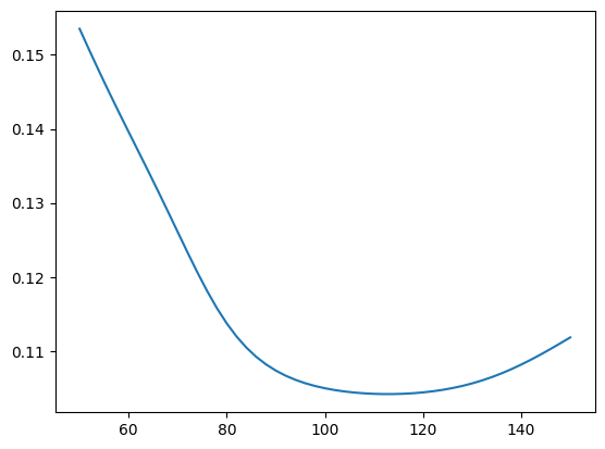
spots = np.linspace(50, 150, 51)
implied_vols = []
for S in spots:
    market = Market(S, market.r, market.q)
    target_price = merton_price(market, model, vanilla)
    implied_vols.append(compute_implied_vol(*market, vanilla, target_price))
implied_vols = np.array(implied_vols)

plt.plot(spots, implied_vols)

[<matplotlib.lines.Line2D at 0x137b69070>]

merton_price(market, model, vanilla)

5.056358953867849

def generate_paths(market, model, contract, num_paths, num_steps):
    S_0, r, q = market
    σ, λ, μ, δ = model
    m = np.exp(a + 0.5 * b**2) - 1
    retval = [np.ones((num_paths,)) * S_0]
    X = np.log(retval[0])
    schedule = np.linspace(0, contract.T, num_steps + 1)
    W = norm.rvs(size=(num_steps, num_paths))
    W_Λ = norm.rvs(size=(num_steps, num_paths))
    t = 0.0
    for i in range(num_steps):
        Δt = schedule[i + 1] - schedule[i]
        t = t + Δt
        sqrt_Δt = np.sqrt(Δt)
        Λ = poisson.rvs(λ * Δt, size=(num_paths))
        X = X + (r - q - 0.5 * σ**2 - λ * m) * Δt + σ * sqrt_Δt * W[i, :] \
              + Λ * μ + np.sqrt(Λ) * δ * W_Λ[i, :]
        retval.append(np.exp(X))
    return np.vstack(retval)

paths = generate_paths(market, model, vanilla, 10000, 1000)
S_T = paths[-1]
np.exp(-market.r * vanilla.T) * np.maximum(S_T - vanilla.K, 0).mean()

4.975385428435133