In this post we tackle the quite classical MNIST digit recognition problem. This is a relatively simple machine vision task: if we limit ourselves to numbers written in black on a white background, what we have are black or white pixels on a small image. There are only ten numbers, so this is a classification task of modest difficulty, and it is also quite important per se.
Let’s start with a few imports:
import matplotlib.pyplot as plt
import numpy as np
import torch
from torch import nn
import torch.nn.functional as F
from torchvision import datasets, transforms
To run the code on both CPUs and GPUs, we setup a device variable, automatically set to cuda if our system has been configured as such, or to cpu otherwise. Using GPUs isn’t a gigantic boost in this case, but it’s faster and will be useful for more complicated problems.
device = torch.device('cuda:0' if torch.cuda.is_available() else 'cpu:0')
print(f"Device: {device}")
Device: cpu:0
We transform input values in the $[0, 1]$ range into $[-1, 1]$ by subtracting the mean of $0.5$. Values that are zero become -1, and values that are 1 stay at that level. Normalization helps to reduce the skewness of the data. The resize to 28 pixels isn’t required with the training and validation data, but will be handy later on to test the network on custom images of different sizes. The variable batch_size is set here to 512.
transform = transforms.Compose([transforms.Resize(28, 1),
                                transforms.ToTensor(),
                                transforms.Normalize((0.5,), (0.5,))])
training_dataset = datasets.MNIST(root='./data', train=True, transform=transform, download=True)
validation_dataset = datasets.MNIST(root='./data', train=False, transform=transform, download=True)

batch_size = 512
training_loader = torch.utils.data.DataLoader(dataset=training_dataset, batch_size=batch_size, shuffle=True)
# no need to shuffle the validation data as we don't train on it
validation_loader = torch.utils.data.DataLoader(dataset=validation_dataset, batch_size=batch_size, shuffle=False)
def im_convert(tensor):
    image = tensor.clone().detach().numpy()
    image = image.transpose(1, 2, 0)
    image = image * np.array([0.5, 0.5, 0.5]) + np.array([0.5, 0.5, 0.5])
    image = image.clip(0, 1)
    return image
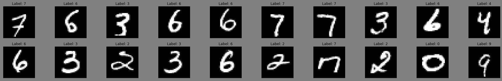
To explore the dataset, we plot a few of the images and the corresponding labels.
dataiter = iter(training_loader)
images, labels = dataiter.next()
print(f"Image shape: {images[0].shape[0]} x {images[0].shape[1]} x {images[0].shape[2]}\n")
fig = plt.figure(figsize=(25, 4))

for idx in range(20):
    ax = fig.add_subplot(2, 10, idx + 1, xticks=[], yticks=[])
    plt.imshow(im_convert(images[idx]))
    ax.set_title(f"Label: {labels[idx].item()}")
fig.set_facecolor('grey')
plt.tight_layout()
Image shape: 1 x 28 x 28
The model that we use is the classical LeNet model. Proposed in 1989 by Yann LeCun at al., it is by today’s standards (and today’s hardware as well) a simple convolutional neural network, yet it performs very well on this task. The Handwritten Digit Recognition with a Back-Propagation Network paper also describes nicely the engineering tasks needed to generate such data.
class LeNet(nn.Module):
    def __init__(self):
        super().__init__()
        # the data on the edges is just dark pixels so it doesn't matter if we lose it
        # hence, no padding, and after each convolutional layer
        # the image size becomes smaller
        # the input layer has 1 layer, 20 features, kernel size is 5, strike is 1
        self.conv1 = nn.Conv2d(1, 20, 5, 1)
        # the second layer has 20 channels and 50 features
        self.conv2 = nn.Conv2d(20, 50, 5, 1)
        # the 50 is the output size of conv2, 4 * 4 is because
        # we have no padding in conv1 (so size is 28 - 4 = 24),
        # then a pooling layer (size 24 / 2 = 12), then conv2
        # (12 - 4 = 8) and another pooling layer (8 / 2 = 4)
        self.fc1 = nn.Linear(4 * 4 * 50, 500)
        self.fc2 = nn.Linear(500, 10)
        # dropout layer
        self.dropout1 = nn.Dropout(0.5)

    def forward(self, x):
        x = F.relu(self.conv1(x))
        x = F.max_pool2d(x, 2, 2)
        x = F.relu(self.conv2(x))
        x = F.max_pool2d(x, 2, 2)
        # flatten to pass it to the fully connected layer
        x = x.view(-1, 4 * 4 * 50)
        x = F.relu(self.fc1(x))
        x = self.dropout1(x)
        x = self.fc2(x)
        # no activation function because we use the cross entropy loss
        return x
model = LeNet().to(device)
model
LeNet(
  (conv1): Conv2d(1, 20, kernel_size=(5, 5), stride=(1, 1))
  (conv2): Conv2d(20, 50, kernel_size=(5, 5), stride=(1, 1))
  (fc1): Linear(in_features=800, out_features=500, bias=True)
  (fc2): Linear(in_features=500, out_features=10, bias=True)
  (dropout1): Dropout(p=0.5, inplace=False)
)
criterion = nn.CrossEntropyLoss().to(device)
optimizer = torch.optim.Adam(model.parameters(), lr=0.001)
%%time
epochs = 12
running_loss_history = []
running_corrects_history = []
val_running_loss_history = []
val_running_corrects_history = []

for epoch in range(epochs):
    running_loss = 0.0
    running_corrects = 0
    val_running_loss = 0.0
    val_running_corrects = 0

    for inputs, labels in training_loader:
        inputs = inputs.to(device)
        outputs = inputs.to(device)
        labels = labels.to(device)
        outputs = model(inputs)
        loss = criterion(outputs, labels)
        optimizer.zero_grad()
        loss.backward()
        optimizer.step()

        _, preds = torch.max(outputs, 1)
        running_loss += loss.item()
        running_corrects += torch.sum(preds == labels.data)
    else:
        # validation dataset. Using no_grad() puts to False all the requires_grad flags
        # within the scope of the with
        with torch.no_grad():
            for val_inputs, val_labels in validation_loader:
                val_inputs = val_inputs.to(device)
                val_labels = val_labels.to(device)
                val_outputs = model(val_inputs)
                val_loss = criterion(val_outputs, val_labels)

                _, val_preds = torch.max(val_outputs, 1)
                val_running_loss += val_loss.item()
                val_running_corrects += torch.sum(val_preds == val_labels.data)

        epoch_loss = running_loss / len(training_loader) / batch_size
        running_loss_history.append(epoch_loss)
        running_acc = running_corrects.float() / len(training_loader) / batch_size
        running_corrects_history.append(running_acc)

        val_epoch_loss = val_running_loss / len(validation_loader) / batch_size
        val_running_loss_history.append(val_epoch_loss)
        val_running_acc = val_running_corrects.float() / len(validation_loader) / batch_size
        val_running_corrects_history.append(val_running_acc)

        print(f'Epoch: {epoch}, training loss: {epoch_loss:.4f}, acc: {running_acc:.4f}, val acc: {val_running_acc:.4f}')
Epoch: 0, training loss: 0.0008, acc: 0.8724, val acc: 0.9455
Epoch: 1, training loss: 0.0002, acc: 0.9655, val acc: 0.9563
Epoch: 2, training loss: 0.0001, acc: 0.9750, val acc: 0.9615
Epoch: 3, training loss: 0.0001, acc: 0.9779, val acc: 0.9646
Epoch: 4, training loss: 0.0001, acc: 0.9814, val acc: 0.9653
Epoch: 5, training loss: 0.0001, acc: 0.9829, val acc: 0.9661
Epoch: 6, training loss: 0.0001, acc: 0.9841, val acc: 0.9671
Epoch: 7, training loss: 0.0000, acc: 0.9850, val acc: 0.9679
Epoch: 8, training loss: 0.0000, acc: 0.9864, val acc: 0.9668
Epoch: 9, training loss: 0.0000, acc: 0.9868, val acc: 0.9674
Epoch: 10, training loss: 0.0000, acc: 0.9874, val acc: 0.9676
Epoch: 11, training loss: 0.0000, acc: 0.9880, val acc: 0.9676
Wall time: 7min 55s
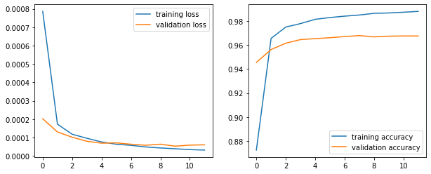
fig, (ax0, ax1) = plt.subplots(ncols=2, figsize=(10, 4))
ax0.plot(running_loss_history, label='training loss')
ax0.plot(val_running_loss_history, label='validation loss')
ax0.legend()

ax1.plot(running_corrects_history, label='training accuracy')
ax1.plot(val_running_corrects_history, label='validation accuracy')
ax1.legend();
Scikit-learn’s classification_report builds a text report showing the main classification metrics. To use it, we firsts define a new DataLoader that has one batch and compute the predictions. We could have used the loader we already have for the validation set, but since it’s a small dataset we can afford to load it entirely in memory.
import sklearn
from sklearn import metrics
loader = torch.utils.data.DataLoader(dataset=validation_dataset, batch_size=len(validation_dataset), shuffle=False)
for X, y in loader:
    output = model(X)
    _, y_pred = torch.max(output, 1)
The classification report gives the precision, recall, F1-score and support.
print(metrics.classification_report(y, y_pred))
              precision    recall  f1-score   support

           0       0.99      1.00      1.00       980
           1       1.00      1.00      1.00      1135
           2       0.98      1.00      0.99      1032
           3       0.99      0.99      0.99      1010
           4       0.99      0.99      0.99       982
           5       0.99      0.99      0.99       892
           6       1.00      0.99      0.99       958
           7       1.00      0.98      0.99      1028
           8       0.99      0.99      0.99       974
           9       0.98      0.99      0.99      1009

    accuracy                           0.99     10000
   macro avg       0.99      0.99      0.99     10000
weighted avg       0.99      0.99      0.99     10000
The scikit-learn plot_confusion_matrix requires a classifier we don’t have. It is easy to build one, but it is also simple to perform the operation of that method here.
cm = metrics.confusion_matrix(y, y_pred)

display_labels = sklearn.utils.multiclass.unique_labels(y, y_pred)

fig, ax = plt.subplots(figsize=(8, 8))
disp = metrics.ConfusionMatrixDisplay(confusion_matrix=cm,
                                  display_labels=display_labels)
disp.plot(include_values=True,
                     cmap='viridis', ax=ax, xticks_rotation='horizontal',
                     values_format=None, colorbar=True);
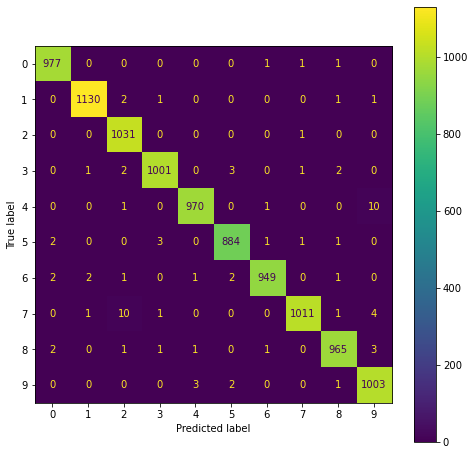
So it looks like a very good fit overall. Perhaps the number 4 is sometimes confused with the number 9, as well as the numbers 7 and 8.
How well does it work on other data? Let’s try on a new image. Open Paint 3D or another similar program and draw a number, then save it to file and pass it to the network. Note that the background should be black and the digit white, with other color combinations creating confusion to the model. Non-white colors will be converted to some shade of gray, possibly causing wrong predictions. Also, the image shape should be square to avoid resizing problems. Here I have used a $56 \times 56$ image, resized to $28\times 28$; larger images may not be resized equally well.
from PIL import Image
The digit I draw is saved in file five.png and is shown on the left. We need to remove the color layers by converting it to black-and-white, as well as resize it. The resulting image is shown on the right – the edges of the number look less sharp.
fig, (ax0, ax1) = plt.subplots(ncols=2, figsize=(8, 4))
img = Image.open('./five.png')
ax0.imshow(img)
ax0.set_xticks([])
ax0.set_yticks([])

img = img.convert('1')
img = transform(img)
ax1.imshow(im_convert(img))
ax1.set_xticks([])
ax1.set_yticks([]);

To test the model we only need to add an additional dimension, as the model accepts tensors of dimension four, and look for the position of the maximum.
output = model(img.unsqueeze(1).to(device))
_, pred = torch.max(output, 1)
print(f"Prediction is: {pred.item()}")
Prediction is: 5
So it looks like it works! However, if your image has colors, or a different background, or the original image size is much larger than $28 \times 28$, then the model may not work.