An autoencoder is a type of neural network that is trained to attempt to copy its inputs into its outputs. Given an input $X \in \mathbb{R}^n$ and two functions $f: \mathbb{R}^n \rightarrow \mathbb{R}^m$ and $g: \mathbb{R}^m \rightarrow \mathbb{R}^n$, they compute $\hat{X} = g(f(X))$ and aim for $Y \approx X$ by making a certain loss function $\mathcal{L}(X, \hat{X})$ as small as possible. We need $m \ll n$, as for $m \ge n$ one can simply take identity functions and perform a trivial transformation.
The function $f$ is called the encoder and $g$ the decoder, with $Z = f(X)$ the code in which a vector $X$ is transformed. The hope is that training will result in the codes $Z$ taking on useful properties, for example removing the noise on $X$ or perform a dimensionality reduction. The vectors $Z$ are often called the latent vectors, which is how we will call them here.
The simplest kind of autoencoder has one layer, linear activations, and squared error loss,
\[\mathcal{L}(X, \hat{X}) = \|X - \hat{X}\|^2.\]This computes $\hat{X} = U V X$, with $U$ and $V$ two matrices. This is a linear function; if $m \ge n$ we can shoose $U$ and $V$ such that $U V = I$, which is not very interesting. If instead $m \ll n$ the encoder is reducing the dimensionality; the output $\hat{X}$ must lie in the column space of $U$. This is equivalent to principal component analysis, or PCA.
The idea of autoencoders is to go a step further and add nonlinearities to project the data not on a subspace, but on a nonlinear manifold. As such, they are more powerful than PCA for a given dimensionality. The learning is unsupervised – they try to reconstruct the inputs from the inputs themselves.
In this article we look at autoencoders as tools for dimensionality reduction. Most of the tutorials on autoencoders do so on images, which are a very important application of generative machine learning models. Here, instead, we will work with mathematical functions and in particular with the well-known the probability density function of the normal distribution,
\[\varphi(x; μ, σ) = \frac{1}{\sigma \sqrt{2 \pi}} \exp \left(-\frac{1}{2}\left( \frac{x - \mu}{\sigma} \right)^2 \right).\]This function has two parameters, $\mu$ and $\sigma$, apart from the input variable $x$. What we do is to create a grid of points $[x_1, x_2, \ldots, x_n]$ on which we will sample $\varphi(x; μ, σ)$ for given values of $\mu$ and $\sigma$. The grid is fixed and identical for all values of the parameters. The sampled function on the grid has length $n$ and is the quantity that the autoencoder will operator upon. Ideally the autoencoder should learn how to represent this function on the provided grid. We expect a latent space of dimension two to suffice, and we will check that.
We start by creating the environment for the code:
conda create --name normal-distribution python==3.9 --no-default-packages -y
conda activate normal-distribution
pip install torch numpy scipy matplotlib seaborn
We import the required packages:
from matplotlib.patches import Rectangle
import matplotlib.pyplot as plt
import numpy as np
from scipy.optimize import minimize
import seaborn as sns
import torch
import torch.nn as nn
import torch.nn.functional as F
import torch.utils
from torch.utils.data import Dataset, DataLoader
import torch.distributions
We specify a device such that we can use CPUs, GPUs, or anything else supported by PyTorch. The CPU will suffice given the small size of what we are doing.
device = 'cuda' if torch.cuda.is_available() else 'cpu'
print(f"Using device {device}.")
Using device cpu.
The first phase is the generation of the training dataset. The dataset is composed by a vector sampling out target function, on a predefined grid, for some values of $\mu$ and $\sigma$ that are given by a random number generator. We have to limit ourselves to a range of the parameters as we can’t cover them all: we assume $-3 \le \mu \le 3$ and $1/2 \le \sigma \le 3$, while the grid is a discretized uniformly over the $[-5, 5]$ interval.
uniform_dist_μ = torch.distributions.uniform.Uniform(-3.0, 3.0)
uniform_dist_σ = torch.distributions.uniform.Uniform(0.5, 3.0)
We can easily generate as many entries for the training dataset as we want; 100’000 seems a reasonable choice and provides good results. The function $\varphi(x)$ is defined in target_func; a simple for loop fills the input dataset X.
num_inputs = 100_000
num_points = 1_000

grid = torch.linspace(-5.0, 5.0, num_points)

def target_func(x, μ, σ):
    return 1 / np.sqrt(2 * np.pi) / σ * np.exp(-0.5 * (x - μ)**2 /  σ**2)
torch.manual_seed(0)
X, Y = [], []
for _ in range(num_inputs):
    μ = uniform_dist_μ.sample()
    σ = uniform_dist_σ.sample()
    X.append(target_func(grid, μ, σ))
    Y.append([μ, σ])
X = torch.vstack(X)

assert X.shape[0] == num_inputs
assert X.shape[1] == num_points
assert X.isnan().sum() == 0.0
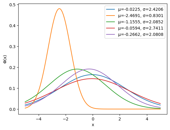
Plotting a few entries of the dataset shows what we have. For the selected parameter ranges, the functions are smooth, yet potentially with large gradients when $\sigma$ is small.
for x, (μ, σ) in zip(X[:5], Y[:5]):
    plt.plot(grid, x, label=f'μ={μ.item():.4f}, σ={σ.item():.4f}')
plt.legend()
plt.xlabel('x')
plt.ylabel('Φ(x)');
The architecture of the encoder is quite simple: a classical sequential network with four layers and tanh activation function.
class Encoder(nn.Module):

    def __init__(self, num_inputs, latent_dims, num_hidden):
        super().__init__()
        self.linear1 = nn.Linear(num_inputs, num_hidden)
        self.linear2 = nn.Linear(num_hidden, num_hidden)
        self.linear3 = nn.Linear(num_hidden, num_hidden)
        self.linear4 = nn.Linear(num_hidden, latent_dims)

    def forward(self, x):
        x = torch.tanh(self.linear1(x))
        x = torch.tanh(self.linear2(x))
        x = torch.tanh(self.linear3(x))
        return self.linear4(x)
The decoder is symmetric and quite simple as well. As we will see, this suffices for our goals so we won’t try more complicated architectures. Since the output is a probability density, we can use RELU to remove negative values from $\hat{X}$.
class Decoder(nn.Module):

    def __init__(self, num_inputs, latent_dims, num_hidden):
        super().__init__()
        self.linear1 = nn.Linear(num_inputs, num_hidden)
        self.linear2 = nn.Linear(num_hidden, num_hidden)
        self.linear3 = nn.Linear(num_hidden, num_hidden)
        self.linear4 = nn.Linear(num_hidden, num_points)

    def forward(self, z):
        z = torch.tanh(self.linear1(z))
        z = torch.tanh(self.linear2(z))
        z = torch.tanh(self.linear3(z))
        return torch.relu(self.linear4(z))
The autoencoder simply composes the encoder and the decoder, passing the input data through the former and then the latter.
class Autoencoder(nn.Module):

    def __init__(self, num_points, latent_dims, num_hidden):
        super().__init__()
        self.encoder = Encoder(num_points, latent_dims, num_hidden)
        self.decoder = Decoder(num_points, latent_dims, num_hidden)

    def forward(self, x):
        z = self.encoder(x)
        x_hat = self.decoder(z)
        return x_hat


def init_weights(m):
    if isinstance(m, nn.Linear):
        torch.nn.init.xavier_uniform_(m.weight)
        m.bias.data.fill_(0.01)
We are almost ready to do the training. A small wrapper to the Dataset class is used such that we can define a DataLoader and specify the batch size (here, 256) and shuffling.
class FuncDataset(Dataset):

    def __init__(self, X):
        self.X = X

    def __len__(self):
        return len(self.X)

    def __getitem__(self, idx):
        return self.X[idx]
data_loader = DataLoader(FuncDataset(X), batch_size=256, shuffle=True)
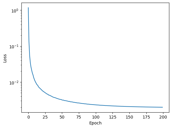
The training goes through the specified epochs; for each epoch we iterate over the batches, compute $\hat{X}$ given $X$ and evaluate the loss function, whose gradients are used by the optimizer to converge.
def train(autoencoder, data_loader, epochs, lr, gamma, print_every):
    optimizer = torch.optim.Adam(autoencoder.parameters(), lr=lr)
    scheduler = torch.optim.lr_scheduler.ExponentialLR(optimizer, gamma=gamma)
    history = []
    for epoch in range(1, epochs + 1):
        last_lr = scheduler.get_last_lr()
        total_loss = 0.0
        for x in data_loader:
            x = x.to(device)  # to GPU if necessary
            optimizer.zero_grad()
            x_hat = autoencoder(x)
            loss = F.mse_loss(x, x_hat)
            loss.backward()
            optimizer.step()
            total_loss += loss.item()
        scheduler.step()
        if epoch % print_every == 0:
            print(f"Epoch: {epoch:3d}, lr: {last_lr[0]:.4e}, avg loss: {total_loss:.4f}")
        history.append(total_loss)
    return history
torch.manual_seed(0)
latent_dims = 2
autoencoder = Autoencoder(num_points, latent_dims=latent_dims, num_hidden=16).to(device)
autoencoder.apply(init_weights)
history = train(autoencoder, data_loader, epochs=100, lr=1e-3, gamma=0.98, print_every=10)
Epoch:  10, lr: 8.3375e-04, avg loss: 0.0119
Epoch:  20, lr: 6.8123e-04, avg loss: 0.0063
Epoch:  30, lr: 5.5662e-04, avg loss: 0.0046
Epoch:  40, lr: 4.5480e-04, avg loss: 0.0037
Epoch:  50, lr: 3.7160e-04, avg loss: 0.0033
Epoch:  60, lr: 3.0363e-04, avg loss: 0.0029
Epoch:  70, lr: 2.4808e-04, avg loss: 0.0027
Epoch:  80, lr: 2.0270e-04, avg loss: 0.0025
Epoch:  90, lr: 1.6562e-04, avg loss: 0.0024
Epoch: 100, lr: 1.3533e-04, avg loss: 0.0023
Epoch: 110, lr: 1.1057e-04, avg loss: 0.0023
Epoch: 120, lr: 9.0345e-05, avg loss: 0.0022
Epoch: 130, lr: 7.3818e-05, avg loss: 0.0022
Epoch: 140, lr: 6.0315e-05, avg loss: 0.0021
Epoch: 150, lr: 4.9282e-05, avg loss: 0.0021
Epoch: 160, lr: 4.0267e-05, avg loss: 0.0021
Epoch: 170, lr: 3.2901e-05, avg loss: 0.0020
Epoch: 180, lr: 2.6882e-05, avg loss: 0.0020
Epoch: 190, lr: 2.1965e-05, avg loss: 0.0020
Epoch: 200, lr: 1.7947e-05, avg loss: 0.0020
plt.semilogy(history)
plt.xlabel('Epoch')
plt.ylabel('Loss');
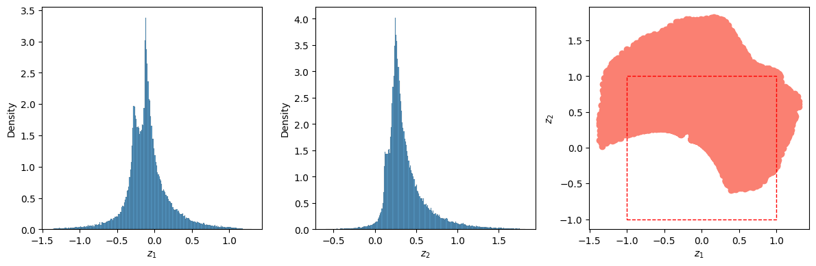
It is important at this point to look at the latent space. as we have no control on how to is defined and which shape it has. To do that, we apply the encoder to all out dataset and store the results in the Z array; we then plot the distribution of $Z_1$ and $Z_2$, as well as all the points $(Z_1, Z_2)$. From the first two graphs we can appreciate that the first latent dimension goes from about -1.5 to 1.5, while the second from -0.5 to about 1.5. The scatter plot on the right is the most interesting: the points have a peculiar shape and are not well distributed around the origin. The dashed red line represents the $(-1, 1) \times (-1, 1)$ square, and we can see that the lower part of the square has not been covered while training. This means that points generated by the decoder when $z_1=-1$ and $z_2=-1$ will be based on extrapolation rather than interpolation and will probably be of poor quality.
Z = []
for entry in X:
    Z.append(autoencoder.encoder(entry.to(device)).cpu().detach().numpy())
Z = np.array(Z)

fig, (ax0, ax1, ax2) = plt.subplots(figsize=(12, 4), ncols=3)
sns.histplot(Z[:, 0], ax=ax0, stat='density')
sns.histplot(Z[:, 1], ax=ax1, stat='density')
ax2.scatter(Z[:, 0], Z[:, 1], color='salmon')
ax0.set_xlabel('$z_1$')
ax1.set_xlabel('$z_2$')
ax2.set_xlabel('$z_1$'); ax2.set_ylabel('$z_2$')
ax2.add_patch(Rectangle((-1, -1), 2, 2, linestyle='dashed', color='red', alpha=1, fill=None))
fig.tight_layout()
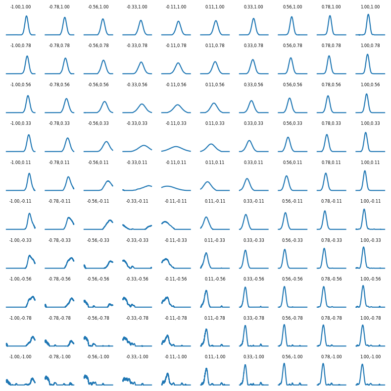
We can also plot the reconstructed function over a few points in the $[-1, 1] \times [-1, 1]$ square of the picture above. We do this on a 10 by 10 grid, showing the result of the decoder for several values of $Z_1$ and $Z_2$ in the square region. In the zone that was not well covered in the trainig phase we expect poor results, and indeed the results aren’t very meaningful there; otherwise we can see the shape of $\hat{X}$ changing with the two parameters as we would expect from a normal distribution.
n = 10
fig, axes = plt.subplots(nrows=n, ncols=n, figsize=(8, 8), sharex=True, sharey=True)
for i, c_1 in enumerate(np.linspace(-1, 1, n)):
    for j, c_2 in enumerate(np.linspace(-1, 1, n)):
        y = autoencoder.decoder(torch.FloatTensor([c_1, c_2]).to(device)).detach().cpu()
        axes[n - 1 - j, i].plot(grid, y)
        axes[n - 1 - j, i].axis('off')
        axes[n - 1 - j, i].set_title(f'{c_1:.2f},{c_2:.2f}', fontsize=6)
fig.tight_layout()
Another thing that can be easily done is to search for the latent values that fit a given $X$, that is looking for the $\hat{X}$ that is closest to the specified $X$. To that aim, we define new random values for $\mu$ and $\sigma$ and look for the latent variables that provide the best fit. The search is performed using SciPy’s minimize and is extremely fast.
μ = uniform_dist_μ.sample()
σ = uniform_dist_σ.sample()

print(f'Params for the test: μ={μ.item():.4f}, σ={σ.item():.4f}\n')

X_target = target_func(grid, μ, σ).numpy()

def func(x):
    X_pred = autoencoder.decoder(torch.FloatTensor(x).to(device))
    X_pred = X_pred.cpu().detach().numpy()
    diff = np.linalg.norm(X_target - X_pred).item()
    return diff

res = minimize(func, [0.0, 0.0], method='Nelder-Mead')
print(res)
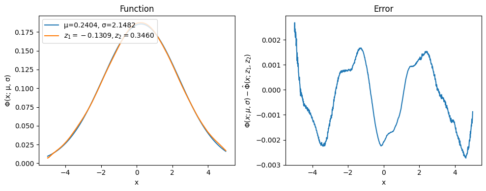
Params for the test: μ=0.2404, σ=2.1482

       message: Optimization terminated successfully.
       success: True
        status: 0
           fun: 0.04326499626040459
             x: [-1.309e-01  3.460e-01]
           nit: 53
          nfev: 103
 final_simplex: (array([[-1.309e-01,  3.460e-01],
                       [-1.310e-01,  3.460e-01],
                       [-1.309e-01,  3.461e-01]]), array([ 4.326e-02,  4.327e-02,  4.327e-02]))
Plotting the results shows quite a good agreement between the exact solution and the one produced by the decoder; increasing the size of the training dataset or the number of epoch would increase the quality.
X_pred = autoencoder.decoder(torch.FloatTensor(res.x).to(device)).cpu().detach().numpy()
fig, (ax0, ax1) = plt.subplots(figsize=(10, 4), ncols=2)
ax0.plot(grid, X_target, label=f'μ={μ.item():.4f}, σ={σ.item():.4f}')
ax0.plot(grid, X_pred, label=f'$z_1={res.x[0].item():.4f}, z_2={res.x[1].item():.4f}$')
ax0.legend(loc='upper left')
ax1.plot(grid, X_target - X_pred)
ax0.set_xlabel('x')
ax0.set_ylabel('Φ(x; μ, σ)')
ax0.set_title('Function')
ax1.set_xlabel('x')
ax1.set_ylabel('$Φ(x; μ, σ) - \hat Φ(x; z_1, z_2)$')
ax1.set_title('Error')
fig.tight_layout()
We conclude by noting that autoencoders are not generative models, so they don’t define a distribution: the latent space they convert their inputs may not be continuous or allow for easy interpolation, especially with large number of latent dimensions. Choosing the correct number of latent dimensions is another problem as well – here we knew it, in general this needs experimenting.