This article is the first of a small series on the usage of artificial neural networks to approximate the solution of partial differential equations. Here we focus on ordinary differential equations (ODEs), in the following ones on partial differential equations (PDEs) and partial-integral differential equations (PIDEs).
Differential equations are ubiquitous, with many applications. They are common and established subject of research, with solid and well-developed mathematical theories and a variety of numerical methods to approximate their solutions. Typically, people use finite differences, finite volumes, finite elements, spectral elements, boundary elements, radial basis functions or even Monte Carlo mehods. A less known approach is what we consider here instead: least-squares methods. This approach is quite old – the article A review of least‐squares methods for solving partial differential equations by Ernest Eason was published in 1976 and contains 241 references on the subject – however it has fallen out of sight until recently. The idea is quite simple, so let’s go through it. We want to find the solution of
\begin{align}
L u & = f \quad \text{in } \Omega
B u & = g \quad \text{on } \partial \Omega
\end{align}
where $L$ is a differential operator that specifies the behavior in the interior of the domain $\Omega$ and $B$ is an operator that defines the boundary conditions. We assume that the problem is well posed such that a solution exists and is unique. As said above here we focus on an operator $L$ with derivatives to one variable only such that $B$ specifies the initial conditions. To simplify the notation and without loss of generality, we can write
\begin{align}
\frac{d u(t)}{dt} & = F(t, u(t)) \quad t \in [0, T]
u(0) & = u_0.
\end{align}
The idea is to approximate the solution $u(t)$ with a function $\hat{u}(t; \omega)$ that depends on some parameters $\omega \in \mathbb{R}^n$. If $\hat{u}$ is regular enough, on some points ${0 \le t_i \le T, i =1,\ldots,m}$ we have $m$ generally nonzero residuals
\begin{align}
R_i(\omega) & = \left[ \frac{d \hat{u}(t_i; \omega)}{dt} - F(t_i, \hat{u}(t_i; \omega)) \right] \neq 0
\end{align}
that we can minimize in the least-squares sense. That is, our numerical solution will be
$\hat{u}(t; \omega^\star)$, with
\begin{equation}
\omega^\star = argmin \frac{1}{2} \sum_{i=1}^m R_i^2(\omega).
\end{equation}
The above expression (with additional terms involving the boundary conditions as we’ll see) brings us back to the classical machine learning approach of minimizing a loss function over a certain amount of points. This is exactly what we will do, with a $\hat{u}(t; \omega)$ defined as a neural network of some kind.
We start as usual with a few imports.
from abc import abstractmethod
import matplotlib.pylab as plt
import numpy as np
import torch
from torch import nn
from torch.autograd import grad
device = torch.device('cuda:0' if torch.cuda.is_available() else 'cpu:0')
print(f"Device: {device}")
Device: cpu:0
The function $\hat{u}(t; \omega)$ aiming to approximate the solution is give by the Model
and is a simple feedforward network. This will suffice for the problems we are covering here, but more complicated networks could be used as well. We assume that our solution as well as the $F$ term above is potentially a vector of dimension $d$ (that is, $d$ = num_equations in the code below).
class Model(nn.Module):
    def __init__(self, n, num_equations):
        super(Model, self).__init__()
        self.linear1 = nn.Linear(1, n)
        self.linear2 = nn.Linear(n, n)
        self.linear3 = nn.Linear(n, num_equations)
        self.activation = nn.Sigmoid()
        for m in self.modules():
            if isinstance(m, nn.Linear):
                nn.init.normal_(m.weight, mean=0, std=0.1)

    def forward(self, t):
        u = self.activation(self.linear1(t))
        u = self.activation(self.linear2(u))
        u = self.linear3(u)
        return u
This small utility function will be used later.
def flat(x):
    m = x.shape[0]
    return [x[i] for i in range(m)]
To make things easier to understand, we define the problem we want to solve through a base class, ODEProblem. This step is technically not needed but it makes the methods easier to write and understand. The methods of this base class are:
- the
domain()method that returns a tuple with two elements, $t_B$ and $t_E$, such that $t \in [t_B, t_E]$; - the
initial_conditions()method that returns a vector with the initial conditions for all the equations we have in the system; - the
equations()method returns a vector of size $d$; each element is a pairs, with the left-hand side and the right-hand side evaluated at time $t$.
class ODEProblem:
    @abstractmethod
    def domain(self):
        pass

    @abstractmethod
    def initial_conditions(self):
        pass

    @abstractmethod
    def equations(self, t):
        pass
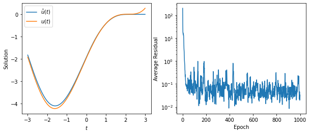
Let’s start from a simple problem with an analytic solution. The single equation is
\[\frac{d}{dt} u(t) + u(t) = t \sqrt[3]{u(t)^2},\]with $u(0) = u_0$. The equation can be solved with the change of variable $u = y^3$, which brings the linear equation
\[3 \frac{d}{d} y(t) + y(t) + t = 0\]whose general solution is
\[y(t) = C e^{-\frac{t}{3}} + t - 3,\]that is
\[u(t) = \left(C e^{-\frac{t}{3}} + t - 3\right)^3.\]The solution exists on $\mathbb{R}$; we use $t \in (-3, 3)$.
class Problem1(ODEProblem):
    def __init__(self, model):
        super().__init__()
        self.t_0 = torch.tensor([[0.0]], dtype=torch.float32, requires_grad=True).to(device)
        self.u_0 = self.exact_solution(torch.FloatTensor([[-3.0]]).to(device))
        self.model = model

    def domain(self):
        return [-3.0, 3.0]

    def initial_conditions(self):
        return [(self.model(self.t_0), self.u_0)]

    def equations(self, t):
        u = self.model(t)
        u_t = grad(flat(u), t, create_graph=True, allow_unused=True)[0]
        lhs = u_t + u
        rhs = t * torch.pow(torch.abs(u), 2.0 / 3)
        return [(lhs, rhs)]

    def exact_solution(self, t):
        return (1.75 * torch.exp(-t / 3) + t - 3)**3
We are now ready to solve the minimization problem. The idea is to generate $n$ points randomly in the domain of integration and evaluate the residuals on those points to define the loss function. We always include the residual at the origin, to make sure the initial condition is correctly considered. As usual we split the optimization step using mini-batches, then run a certain number of epochs. The procedure is wrapped into a function, as we will use it for more than one problem.
def integrate(problem, n, batch_size, num_epochs, lr, boundary_weight, print_every=1_000):
    assert n > 0 and batch_size > 0
    assert num_epochs > 0
    assert lr > 0 and boundary_weight > 0

    num_batches = n // batch_size

    loss_fn = nn.MSELoss().to(device)
    optimizer = torch.optim.Adam(model.parameters(), lr=lr)
    domain = problem.domain()
    t_0 = torch.FloatTensor([[domain[0]]]).to(device)
    t_1 = torch.FloatTensor([[domain[1]]]).to(device)

    history = []
    for epoch in range(num_epochs):
        total_loss = 0.0
        for _ in range(num_batches):
            optimizer.zero_grad()
            t = t_0 + (t_1 - t_0) * torch.rand((1, batch_size), requires_grad=True, dtype=torch.float32).to(device)
            t = t.reshape(-1, 1)
            loss = 0.0
            for (lhs, rhs) in problem.equations(t):
                loss += loss_fn(lhs, rhs)
            for (lhs_ic, rhs_ic) in problem.initial_conditions():
                loss += boundary_weight * loss_fn(lhs_ic, rhs_ic)
            loss.backward()
            optimizer.step()
            total_loss += loss.detach().cpu().numpy()
        history.append(total_loss)
        if print_every is not None and (epoch + 1) % print_every == 0:
            print(f"Epoch {epoch + 1}: loss = {total_loss:e}")

    return history
model = Model(n=32, num_equations=1).to(device)
problem = Problem1(model)
history = integrate(problem, 1_024, 64, 1_000, 1e-1, 10.0, print_every=None)
t = torch.linspace(*problem.domain(), 201).reshape(-1, 1).to(device)
u_hat = model(t).squeeze()
u_exact = problem.exact_solution(t)
fig, (ax0, ax1) = plt.subplots(figsize=(10, 4), ncols=2)
ax0.plot(t.detach().cpu(), u_hat.detach().cpu(), label='$\hat{u}(t)$')
ax0.plot(t.detach().cpu(), u_exact.detach().cpu(), label='$u(t)$')
ax0.set_xlabel('$t$')
ax0.set_ylabel('Solution')
ax0.legend()
ax1.semilogy(history)
ax1.set_xlabel('Epoch')
ax1.set_ylabel('Average Residual');
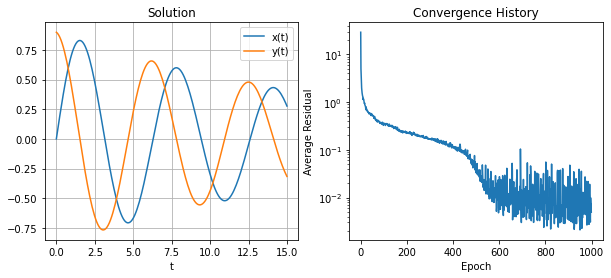
The approach is easily extended to vector system. We consider the damped pendulum
\[\ddot{z}(t) = -\kappa z(t) -\alpha \dot{z}(t),\]converted into a system of two equations of order one,
\[\begin{pmatrix} \dot{z}(t) \\ \ddot{z}(t) \end{pmatrix} = \begin{pmatrix} v(t) \\ \kappa z(t) - \alpha v(t), \end{pmatrix}\]where $v(t) = \dot{z}(t)$. For the numerical values, we use $\kappa=1$ and $\alpha=1/10$; the initial conditions are
\[\begin{pmatrix} z(0) \\ v(0) \end{pmatrix} = \begin{pmatrix} 0 \\ 0.9. \end{pmatrix}.\]class PendulumProblem(ODEProblem):
def __init__(self, model):
super().__init__()
self.t_0 = torch.tensor([[0.0]], dtype=torch.float32, requires_grad=True).to(device)
self.model = model
self.u_0 = torch.tensor([[0.0, 0.9]], dtype=torch.float32).to(device)
def domain(self):
return [0.0, 15.0]
def initial_conditions(self):
return [(self.model(self.t_0), self.u_0)]
def equations(self, t):
u = self.model(t)
x, y = u[:, 0], u[:, 1]
x_t = grad(flat(x), t, create_graph=True, allow_unused=True)[0]
y_t = grad(flat(y), t, create_graph=True, allow_unused=True)[0]
return [
(x_t, y.unsqueeze(-1)),
(y_t, (-x - 0.1 * y).unsqueeze(-1)),
]
model = Model(n=32, num_equations=2).to(device)
problem = PendulumProblem(model)
history = integrate(problem, 4_096, 64, 1_000, 1e-02, 10.0, None)
t = torch.linspace(*problem.domain(), 201).reshape(-1, 1).to(device)
u_hat = model(t).detach().cpu().numpy()
t = t.detach().to(device)
fig, (ax0, ax1) = plt.subplots(figsize=(10, 4), ncols=2)
ax0.plot(t, u_hat[:, 0], label='x(t)')
ax0.plot(t, u_hat[:, 1], label='y(t)')
ax0.grid()
ax0.set_xlabel('t')
ax0.legend()
ax0.set_title('Solution')
ax1.semilogy(history)
ax1.set_xlabel('Epoch')
ax1.set_ylabel('Average Residual')
ax1.set_title('Convergence History');
Is this worth it? For ODEs it doesn’t look like. There is a wealth of well-studied, efficient and reliable methods already, so why bother with a new one that is not so easy to use? Classical methods are also easier to use than the approach presented here, which requires quite a few parameters to be tuned, not always in a straightforward manner. Not only, this method does not always yield a good solution and it is difficult to estimate the impact of the parameters on the outcome. However, the idea is novel and interesting, and we’ll see that for PDEs and PIDEs there are some strengths in this approach.