[Updated on April 2023 to include more recent references.]
In this article we look at how to construct non-uniform grids for solving partial differential equations (PDEs). We follow the methodology presented in the book Pricing Financial Instruments: The Finite Difference Method by Domingo Tavella and Curt Randall, chapter 5. A more recent reference is Inserting or Stretching Points in Finite Difference Discretizations by Jherek Healy.
Out focus is on PDEs approximated by means of a finite difference method on simple domains. By ‘simple’ we mean that the computational domain $\Omega \subset \mathbb{R}^d$ is a product of one-dimensional intervals, $\Omega = [x_{1, min}, x_{1, max}] \times [x_{2, min}, x_{2, max}] \times \cdots \times [x_{d, min}, x_{d, max}]$, with each $x_{i, min}$ and $x_{i, max}$ the minimal and maximal coordinate along the $i-th$ dimension. In this case the grid is the product of the PDE grid on each dimension; it will then suffice to consider the grid construction on a given axis, which is what we will do. We will drop the $i$ index for simplicity of notation, so $x_{min}$ and $x_{max}$ will be the minimal and maximal value of the grid we aim to construct.
Without loss of generality, we assume $0 = \xi_1 < \xi_n < \ldots < \xi_n = 1$ to be a uniform discretization with $n$ points, and $g: [x_{min}, x_{max}] \rightarrow [0, 1]$ a transformation function that maps the uniform coordinates $\xi_i$ into the non-uniform one $x_i$. We write
\[\frac{d x(\xi)}{d\xi} = g'(\xi),\]where $g’(\xi)$ tells us how much the grid changes at any given point. By modeling $g’$ we can aim to control the location of the points in the non-uniform grid. Any positive function will do it; our choice will depend on the grid we aim to have.
According to Noye, Computational Techniques for Differential Equations, 1983, page 307, the function $g(\xi)$ should have the following properties:
- $g’(\xi)$ should be finite over the whole interval – if it becomes infinite at some point, then there is poor resolution near that point;
- $g’(\xi)$ must be smaller near at critical point than elsewhere in the interval, which ensures high resolution near the critical point;
- $g’(\xi)$ should never be zero to avoid redundant points in the grid.
The most common case is where we have one point, $x^\star$, around which we want to concentrate the points. In this case a convenient choice for $g’(\xi)$ is
\[g'(\xi) = A \sqrt{\alpha^2 + (x(\xi) - x^\star)^2},\]where $A$ is a constant to be determined, $\alpha$ is a prescribed uniformity parameter, and $x^\star$ is the point around which we want to concentrate the grid points. If $\vert x - x^\star \vert \gg \alpha$, the effective grid spacing is proportional to $x$ (that is, it is logarithmic), however if $\vert x - x^\star\vert \ll \alpha$ then the effective grid spacing is nearly uniform and rougly equal to $\alpha$.
The equation
\[\frac{d x(\xi)}{d\xi} = A \sqrt{\alpha^2 + (x(\xi) - x^\star)^2}\]can be integrated easily,
\[\begin{aligned} \int \frac{dx}{\sqrt{\alpha^2 + (x - x^\star)^2}} & = A \int d \xi \\ % \sinh^{-1}\left( \frac{x - x^\star}{\alpha} \right) & = \xi A + C. \end{aligned}\]The two constants $A$ and $C$ can be computed by imposing the boundary conditions $x(0) = x_{min}$ and $x(1) = x_{max}$,
\[\begin{aligned} \sinh^{-1}\left( \frac{x_{min} - x^\star}{\alpha} \right) & = C \\ % \sinh^{-1}\left( \frac{x_{max} - x^\star}{\alpha} \right) & = A + C. \end{aligned}\]Using
\[\begin{aligned} c_1 & = \sinh^{-1}\left( \frac{x_{min} - x^\star}{\alpha} \right) \\ % c_2 & = \sinh^{-1}\left( \frac{x_{max} - x^\star}{\alpha} \right) \end{aligned}\]we obtain
\[x(\xi) = x^\star + \alpha \sinh^{-1} \left( c_1(\xi - 1) + c_2 \xi \right),\]which is the form we will test. The implementation is straightforward.
import matplotlib.pylab as plt
import numpy as np
import scipy as sp
class SinhTransformation:

    def __init__(self, x_min, x_max, x_star, α):
        assert x_star >= x_min and x_star <= x_max
        assert α > 0
        self.x_min = x_min
        self.x_max = x_max
        self.x_star = x_star
        self.α = α
        self.c_1 = np.arcsinh((self.x_min - self.x_star) / self.α)
        self.c_2 = np.arcsinh((self.x_max - self.x_star) / self.α)

    def __call__(self, ξ):
        assert np.all(ξ >= 0)
        assert np.all(ξ <= 1)
        return self.x_star + self.α * np.sinh(self.c_2 * ξ + self.c_1 * (1 - ξ))

    def __str__(self):
        return f"x_min: {self.x_min}, x_max={self.x_max}, x_*={self.x_star}, α={self.α}"
ξ_grid = np.linspace(0, 1, 25)
def plot_grid(t):
    x_grid = t(ξ_grid)
    for ξ, x in zip(ξ_grid, x_grid):
        plt.vlines(x=ξ, ymin=t.x_min, ymax=x, color='grey')
        plt.hlines(y=x, xmin=0, xmax=ξ, color='salmon')
    plt.plot(ξ_grid, x_grid, '-o')
    plt.axis('square')
    plt.xlabel('Uniform Grid (ξ)')
    plt.ylabel('Stretched Grid (x)')
    plt.title(str(t))
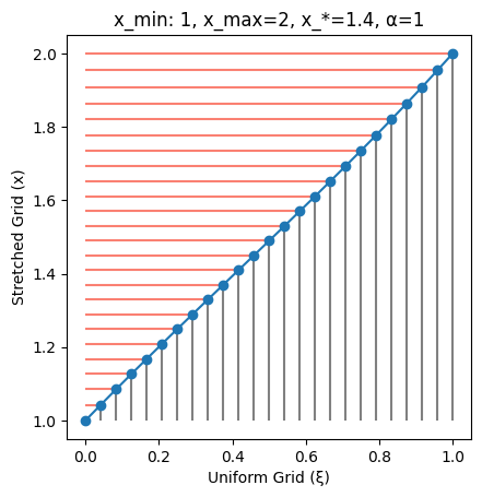
As expected, when $\alpha \gg \vert x - x^\star \vert$ (in this case $\alpha=1$) the grid is almost uniform (though not exactly uniform as said before). On the X-axis we report the uniform grid, indicated by $\xi$ and defined between 0 and 1; the the Y-axis we have the non-uniform grid, indicated by $x$ and defined between $x_{min}$ and $x_{max}$.
plot_grid(SinhTransformation(x_min=1, x_max=2, x_star=1.4, α=1))
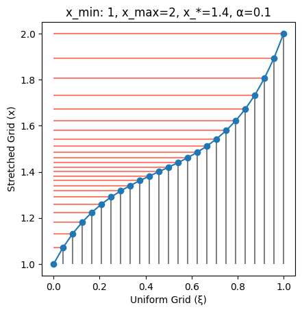
With $\alpha=0.1$ the non-uniformity increases, with points mildly concentrated around $x^\star=1.4$.
plot_grid(SinhTransformation(x_min=1, x_max=2, x_star=1.4, α=0.1))
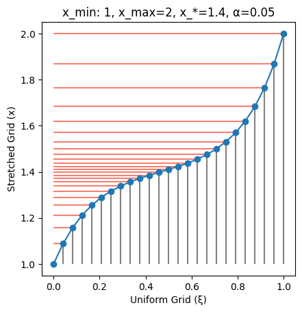
Using $\alpha=0.05$ makes the non-uniformity even more prominent.
plot_grid(SinhTransformation(x_min=1, x_max=2, x_star=1.4, α=0.05))
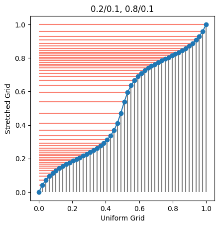
Another case it to have more points around which we want to concentrate the grid. This case is less straightforward. The approach proposed by Tavella and Randall is to use the transformation
\[g'(\xi) = A \left( \Pi_k \frac{1}{\alpha_k^2 + (x(\xi) - x^\star_k)^2} \right)^{-\frac{1}{2}}\]where $A$ is a normalization constant to ensure that $x(1) = x_{max}$, with initial condition $x(0) = x_{min}$. Integrating the equation above means solving an ordinary differential equation (ODE) with two boundary values, which can be done with the shooting method: we assume a value for $A$, integrate, then adapt the value of $A$ to make sure that the condition on $x(1)$ is satisfied. This means that we have a nonlinear solver which requires, at each step, the solution of an ODE. The later is typically solved using explicit methods, like Runge-Kutta. This is clearly more involved than the grid construction with only one concentration point.
from scipy.integrate import solve_ivp
from scipy.optimize import root
class CompositeTransformation:

    def __init__(self, x_star_all, α_all):
        self.x_star_all = x_star_all
        self.α_all = α_all

    def __call__(self, ξ, x, A):
        total = 0.0
        for x_star, α in zip(self.x_star_all, self.α_all):
            total += np.power(α**2 + (x - x_star)**2, -2)
        return A * np.power(total, -0.5)

    def __str__(self):
        retval = []
        for x_star, α in zip(self.x_star_all, self.α_all):
            retval.append(f'{x_star}/{α}')
        return ', '.join(retval)
composite = CompositeTransformation([0.2, 0.8], [0.1, 0.1])
def compute_grid(A):
    sol = solve_ivp(composite, [0, 1], [0], t_eval=np.linspace(0, 1, 1000), args=(A,))
    return sol.y[0]

result = root(lambda A: compute_grid(A)[-1] - 1, [0.1])
assert result.success, result.message
A = result.x[0]
ξ_grid = np.linspace(0, 1, 50)
sol = solve_ivp(composite, [0, 1], [0], t_eval=ξ_grid, args=(A,))
x_grid = sol.y[0]

for ξ, x in zip(ξ_grid, x_grid):
    plt.vlines(x=ξ, ymin=0, ymax=x, color='grey')
    plt.hlines(y=x, xmin=0, xmax=ξ, color='salmon')
plt.plot(ξ_grid, x_grid, '-o')
plt.axis('square')
plt.xlabel('Uniform Grid')
plt.ylabel('Stretched Grid')
plt.title(str(composite));
The above procedure is delicate and doesn’t always converge. Besides, there are only so many points we can move around, so too many concentration points will result in poor coverage of the other areas.