On Modern Portfolio Theory

In this article we address the Model Portfolio Theory proposed in 1952 by the Economics Nobel price winner Harry Markowitz. The key concepts are quite easy. First, Markowitz showed that investors should care about two things - expected return (how much you expect to earn) and risk (measured as variance or standard deviation of returns). Rational investors want higher returns but lower risk. Second, he showed that by combining assets one can reduce overall portfolio risk without sacrificing returns. This happens because assets don’t move in perfect lockstep – when one goes down, another might go up or stay stable. The mathematical relationship between assets is measured by covariance or correlation. Third, the theory gives the set of optimal portfolios that offer the highest expected return for each level of risk, or equivalently, the lowest risk for each level of return. This is called the efficient frontier; any portfolio not on this frontier is suboptimal – you could get better returns for the same risk, or lower risk for the same returns.

import numpy as np
import pandas as pd
import yfinance as yf
import matplotlib.pyplot as plt

First, we download historical data for two major stock market indices, SPY for the S&P 500 (US) and GLD for gold.

tickers = ['SPY', 'GLD']
data = yf.download(tickers, start='2011-01-01', end='2016-01-01', auto_adjust=True)['Close']

[*********************100%***********************]  2 of 2 completed

We now need to compute the annualized daily returns and covariance matrix.

returns = data.pct_change().dropna()
mu = returns.mean() * 252  # 252 trading days per year
sigma = returns.cov() * 252
print(f"Returns: SPY={mu.SPY:.2%}, gold={mu.GLD:.2%}")
sigma

Returns: SPY=12.72%, gold=-4.62%

Ticker	GLD	SPY
Ticker
GLD	0.030703	0.000754
SPY	0.000754	0.023555

We start the portfolio optimization using cvxopt; the constraints are that the sum of weights is one and all the weights are non-negative. This means that we always allocate all the money (no cash holding) and there is no short selling.

from cvxopt import matrix, solvers
solvers.options['show_progress'] = False

n = len(tickers)

P = matrix(sigma.values)
q = matrix(np.zeros(n))
G = matrix(-np.eye(n))
h = matrix(np.zeros(n))
A = matrix(np.ones(n)).T
b = matrix(1.0)

The solution itself is very quick since the problem we are solving is tiny. Of course using thousands of assets would be a different story and will take much longer.

sol = solvers.qp(P, q, G, h, A, b)
weights_min_var = np.array(sol['x']).flatten()

for ticker, weight in zip(tickers, weights_min_var):
    print(f"{ticker}: {weight:.2%}")

portfolio_return = np.dot(weights_min_var, mu)
portfolio_variance = np.dot(weights_min_var, np.dot(sigma.values, weights_min_var))
portfolio_std = np.sqrt(portfolio_variance)

print()
print(f"Expected annual return: {portfolio_return:.2%}%")
print(f"Annual volatility (std dev): {portfolio_std:.2%}%")
print(f"Sharpe ratio (assuming 0% risk-free rate): {portfolio_return/portfolio_std:.2f}")

SPY: 43.23%
GLD: 56.77%

Expected annual return: 5.22%%
Annual volatility (std dev): 11.70%%
Sharpe ratio (assuming 0% risk-free rate): 0.45

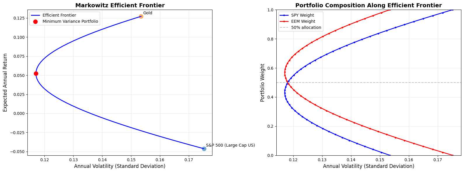
It is interesting to generate the so-called efficient frontier. In our case it means solving for a specific return, then plotting all the portfolio compositions that are generated. We can then graphically see the variance reduction given by the portfolio compared to the individual assets.

target_returns = np.linspace(mu.min(), mu.max(), 50)
efficient_portfolios = []

for target_ret in target_returns:
    # Add constraint for target return
    A_target = matrix(np.vstack([np.ones(n), mu.values]))
    b_target = matrix([1.0, target_ret])
    
    try:
        sol = solvers.qp(P, q, G, h, A_target, b_target)
        if sol['status'] == 'optimal':
            w = np.array(sol['x']).flatten()
            ret = np.dot(w, mu)
            std = np.sqrt(np.dot(w, np.dot(sigma.values, w)))
            efficient_portfolios.append({'return': ret, 'std': std, 'weights': w})
    except:
        pass

ef_returns = [p['return'] for p in efficient_portfolios]
ef_stds = [p['std'] for p in efficient_portfolios]

# Create two subplots
fig, (ax1, ax2) = plt.subplots(1, 2, figsize=(16, 6))

# First plot: Efficient Frontier with assets
ax1.plot(ef_stds, ef_returns, 'b-', linewidth=2, label='Efficient Frontier')
ax1.scatter([portfolio_std], [portfolio_return], color='red', s=100, 
            label='Minimum Variance Portfolio', zorder=5)

# Plot individual assets
for i, ticker in enumerate(tickers):
    ax1.scatter(np.sqrt(sigma.iloc[i, i]), mu.iloc[i], s=100, alpha=0.6)
    ax1.annotate(ticker_names[ticker], (np.sqrt(sigma.iloc[i, i]), mu.iloc[i]), 
                xytext=(5, 5), textcoords='offset points', fontsize=10)

ax1.set_xlabel('Annual Volatility (Standard Deviation)', fontsize=12)
ax1.set_ylabel('Expected Annual Return', fontsize=12)
ax1.set_title('Markowitz Efficient Frontier', fontsize=14, fontweight='bold')
ax1.legend()
ax1.grid(True, alpha=0.3)

# Second plot: Portfolio weights along efficient frontier
spy_weights = [p['weights'][0] for p in efficient_portfolios]
eem_weights = [p['weights'][1] for p in efficient_portfolios]

ax2.plot(ef_stds, spy_weights, 'b-', linewidth=2, label='SPY Weight', marker='o', markersize=3)
ax2.plot(ef_stds, eem_weights, 'r-', linewidth=2, label='EEM Weight', marker='o', markersize=3)
ax2.axhline(y=0.5, color='gray', linestyle='--', alpha=0.5, label='50% allocation')
ax2.set_xlabel('Annual Volatility (Standard Deviation)', fontsize=12)
ax2.set_ylabel('Portfolio Weight', fontsize=12)
ax2.set_title('Portfolio Composition Along Efficient Frontier', fontsize=14, fontweight='bold')
ax2.legend()
ax2.grid(True, alpha=0.3)
ax2.set_ylim([0, 1])

plt.tight_layout()

png