In this article we briefly cover the Stochastic Alpha Beta Rho model, knows as SABR, proposed by Hagan and co-authors. This model is defined by four parameters:
- α is the instantaneous vol;
- ν is the vol of vol;
- ρ is the correlation between the Brownian motions driving the forward rate and the instantaneous vol;
- β is the CEV component for forward rate (determines shape of forward rates, leverage effect and backbone of ATM vol).
β is one of the key parameters and affect many fundamental characteristics of the model. β is the exponent for the forward rate or the CEV exponent and effects the distribution:
- β = 1 represents stochastic lognormal dynamics;
- β = 0 defines stochastic normal dynamics;
- β = ½ defines dynamics that are similar to the ones of the CIR model.
As for the CEV component, β helps capture leverage effect without changing the underlying instantaneous vol (α).
from dataclasses import dataclass, field
import matplotlib.pylab as plt
import numpy as np
from scipy.optimize import root_scalar
from scipy.stats import norm
Φ = norm.cdf
@dataclass
class Market:
    r: float
    q: float
    S_0: float
    T: float
    F_0: float = field(init=False)

    def __post_init__(self):
        self.F_0 = self.S_0 * np.exp((self.r - self.q) * self.T)
@dataclass
class Model:
    α_0: float
    β: float
    ρ: float
    ν: float
@dataclass
class Contract:
    K: float
    T: float
    is_call: bool
def generate_paths(F_0, model, schedule, num_paths):
    N = len(schedule) - 1
    α_0, β, ρ, ν = model.α_0, model.β, model.ρ, model.ν

    F_all, α_all = [np.ones((num_paths,)) * F_0], [np.ones((num_paths,)) * α_0]
    F_t = F_all[0]
    α_t = α_all[0]
    W_F = np.random.randn(N, num_paths)
    W_α_ortho = np.random.randn(N, num_paths)
    W_α = ρ * W_F + np.sqrt(1 - ρ**2) * W_α_ortho

    t = 0.0
    for i in range(N):
        Δt = schedule[i + 1] - schedule[i]
        t = t + Δt
        sqrt_Δt = np.sqrt(Δt)
        F_t = F_t + α_t * np.power(F_t, β) * sqrt_Δt * W_F[i]
        F_t = np.maximum(F_t, 0.0)
        α_t = α_t + ν * α_t * sqrt_Δt * W_α[i]
        F_all.append(F_t)
        α_all.append(α_t)

    return np.vstack(F_all), np.vstack(α_all)
def compute_mc_price(F_T, market, contract):
    df = np.exp(-market.r * contract.T)
    ω = 1.0 if contract.is_call else -1.0
    Π = df * np.maximum(ω * (F_T - contract.K), 0)
    mc_price, mc_std = Π.mean(), Π.std() / np.sqrt(len(F_T))
    return mc_price, mc_std
def compute_sabr_implied_vol(market, model, contract):
    F_0 = market.F_0
    α_0, β, ρ, ν = model.α_0, model.β, model.ρ, model.ν
    K, τ = contract.K, contract.T

    # strike on the forward
    if abs(F_0 - K) < 1e-9:
        I_1 = (1 - β**2) / 24 * 0**2 / np.power(F_0, 2 - 2 * β)
        I_2 = 1 / 4 * ρ * β * ν * α_0 / np.power(F_0, 1 - β)
        I_3 = (2 - 3 * ρ**2) / 24 * ν**2
        σ_ATM = α_0 / np.power(F_0, 1 - β) * (1 + (I_1 + I_2 + I_3) * τ)
        return σ_ATM

    # all other cases
    ζ = ν / α_0 * np.power(F_0 * K, (1 - β) / 2) * np.log(F_0 / K)
    χ = np.log((np.sqrt(1 - 2 * ρ * ζ + ζ**2) + ζ - ρ) / (1 - ρ))
    D_1 = (1 - β)**2 / 24 * (np.log(F_0 / K))**2
    D_2 = (1 - β)**4 / 1920 * (np.log(F_0 / K))**4
    D = np.power(F_0 * K, (1 - β) / 2) * (1 + D_1 + D_2)
    N_1 = (1 - β)**2 / 24 * α_0**2 / np.power(F_0 * K, 1 - β)
    N_2 = ρ * β * ν * α_0 / 4 / np.power(F_0 * K, (1 - β) / 2)
    N_3 = (2 - 3 * ρ**2) / 24 * ν**2
    N = α_0 * ζ / χ * (1 + (N_1 + N_2 + N_3) * τ)
    σ = N / D

    return σ
def compute_analytic_price(F_0, r, σ, contract):
    K, T, is_call = contract.K, contract.T, contract.is_call
    τ = T
    ω = 1.0 if is_call else -1.0
    if τ == 0.0:
        return max(ω * (F_0 - K), 0.0)
    df = np.exp(-r * τ)
    d_plus = (np.log(F_0 / K) + 0.5 * σ**2 * τ) / σ / np.sqrt(τ)
    d_minus = d_plus - σ * np.sqrt(τ)
    return ω * df * (F_0 * Φ(ω * d_plus) - K * Φ(ω * d_minus))
market = Market(r=0.2, q=0.1, S_0=100.0, T=1.0)
model = Model(α_0=0.1, β=1.0, ρ=-0.5, ν=0.25)
t_all = np.linspace(0, market.T, 256)
num_paths = 100_000
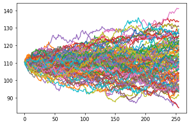
F_all, α_all = generate_paths(market.F_0, model, t_all, num_paths=num_paths)
for i in range(100):
    plt.plot(F_all[:, i])
def compute_implied_vol(F_0, r, σ_0, contract, target_price):
    def inner(σ):
        return compute_analytic_price(F_0, r, σ, contract) - target_price
    try:
        result = root_scalar(inner, x0=σ_0, bracket=[1e-3, 0.5])
    except:
        return np.nan
    return np.nan if not result.converged else result.root
contract = Contract(K=market.F_0, T=market.T, is_call=True)
σ_ATM = compute_sabr_implied_vol(market, model, contract)
width = 3 * σ_ATM * np.sqrt(market.T)
σ_mcs, σ_models = [], []
Ks = np.linspace(market.F_0 * np.exp(-width), market.F_0 * np.exp(width), 101)
for K in Ks:
    contract = Contract(K=K, T=market.T, is_call=K > market.F_0)
    mc_price, mc_std = compute_mc_price(F_all[-1], market, contract)
    σ_models.append(compute_sabr_implied_vol(market, model, contract))
    σ_mcs.append(compute_implied_vol(market.F_0, market.r, σ_ATM, contract, mc_price))
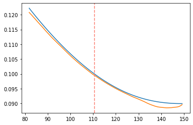
plt.plot(Ks, σ_models)
plt.plot(Ks, σ_mcs)
plt.axvline(x=market.F_0, linestyle='dashed', color='salmon')
<matplotlib.lines.Line2D at 0x1a938d69be0>
Fitting the market data with SABR starts with a selection of β, as different β values give rise to different dynamics, while the other parameters are calibrated. Usually the calibration is a straightforward procedure as the three parameters α, ρ, and ν have different effects on the curve:
- α controls the overall height of the curve;
- ρ controls the curve’s skew;
- ν controls how much smile the curve exhibits.
Because of the widely separated roles these parameters play, the fitted parameter values tend to be very stable, even in the presence of large amounts of market noise.