Bounded Brownian Motion and the Skorokhod Reflection Problem

Bounded Brownian Motion and the Skorokhod Reflection Problem

A common problem in the modelling of systems with stochastic differential equations (SDEs) is to define a diffusion process that is bounded, that is, one that stays within a band $[L, U]$. We start with the discrete case: in a Monte Carlo simulation, we would apply an obvious reflection — if the step overshoots $L$ (or equivalently $U$), we clip it back with a small correction just large enough to pull it back into the band. As $\Delta t \to 0$, the path becomes continuous and the individual corrections $\delta$ shrink to zero individually. But they happen infinitely often: a Wiener process hits any level infinitely often in any time interval. So $\phi^+$ is built from infinitely many infinitesimal pushes — it is a continuous, non-decreasing process that only grows on the set ${t : X_t = L}$.

That set has zero Lebesgue measure (just like any single point does). So $\phi^+$ is a process that increases on a set of times of measure zero. Ordinary calculus has no name for this. That object is the local time.

The boundary push $\phi^+$ must satisfy three conditions simultaneously:

1. Non-decreasing (it only pushes, never pulls)
2. Continuous (the reflected path has no jumps)
3. Only active when $X_t = L$ — it does nothing in the interior

No ordinary process satisfies all three. A process that only moves on a measure-zero set and is still continuous and non-decreasing is, by definition, a singular process — and local time is the canonical example of one. So it is not a modelling choice; it is forced on you by the requirements of the problem.

A Brownian path spends zero Lebesgue time at any fixed level $a$, yet visits it infinitely often. Local time reconciles these two facts by measuring visits in a rescaled sense:

\[L_t^a = \lim_{\varepsilon \to 0} \frac{1}{2\varepsilon} \int_0^t \mathbf{1}_{|W_s - a| < \varepsilon}\, ds.\]

You look at a thin strip of width $2\varepsilon$ around $a$, measure the time spent inside it, then divide by $2\varepsilon$ to get a density. It can be shown that the limit is finite and non-trivial — it is exactly the “intensity” of visits to $a$. This is analogous to a probability density: one cannot assign probability to a single point, but one can assign a density there. Local time is the density of the occupation measure of the path.

The Skorokhod reflection problem makes all of this precise. Given a standard Brownian motion $W_t$ and a starting point $x_0 \in [L, U]$, it asks for a triple $(X_t, \phi^+_t, \phi^-_t)$ such that $X_t$ stays in $[L, U]$, the two boundary processes $\phi^+$ and $\phi^-$ are non-decreasing and continuous, and each only grows when the process is at its respective wall. The solution exists, is unique, and identifies $\phi^+$ and $\phi^-$ as the local times of $X$ at $L$ and $U$. In what follows we develop the theory, derive an exact solution of the associated Fokker-Planck equation, and illustrate everything with Monte Carlo simulations.

1. Local Time

The density interpretation of local time has a precise formulation. For any Borel function $f \geq 0$, the occupation time formula states

\[\int_0^t f(W_s)\, ds = \int_{-\infty}^{+\infty} f(a)\, L_t^a\, da,\]

where $L_t^a$ is the local time of $W$ at level $a$ up to time $t$. This is the Radon–Nikodym derivative of the occupation measure $B \mapsto \int_0^t \mathbf{1}_{W_s \in B}\, ds$ with respect to Lebesgue measure — in other words, exactly the density whose existence the introduction argued for.

Tanaka’s Formula

The cleanest analytical handle on local time comes from applying Itô’s formula to the non-smooth function $x \mapsto (x - a)^+$. Because this function has no classical second derivative at $x = a$, the standard Itô formula must be corrected by a boundary term, and that term is local time. The result is Tanaka’s formula:

\[(W_t - a)^+ = (W_0 - a)^+ + \int_0^t \mathbf{1}_{W_s > a}\, dW_s + \frac{1}{2} L_t^a.\]

Several key properties follow immediately:

• $t \mapsto L_t^a$ is non-decreasing and continuous (a.s.).
• $L_0^a = 0$.
• $L_t^a$ only grows when $W_t = a$: it is a singular process, flat almost everywhere, with all its increase concentrated on the zero-measure set ${t : W_t = a}$.

That last property is precisely what we need to build a bounded process: a push that acts only at the boundary and is invisible everywhere else.

2. The Skorokhod Reflection Problem

One-sided reflection

It is instructive to start with the simpler, one-sided version: keep a Brownian motion non-negative by reflecting it at 0. Given $Y_t = x_0 + W_t$ with $x_0 \geq 0$, find a pair $(X_t, \phi_t)$ such that

1. $X_t = Y_t + \phi_t \geq 0$ for all $t \geq 0$,
2. $\phi_t$ is non-decreasing and continuous, with $\phi_0 = 0$,
3. $\phi$ only increases when $X_t = 0$: $\int_0^\infty \mathbf{1}_{X_t > 0}\, d\phi_t = 0$.

The unique solution is given by the Lévy–Skorokhod formula:

\[\phi_t = \left(-\inf_{s \leq t} Y_s\right)^+, \qquad X_t = Y_t + \phi_t.\]

The process $\phi_t$ is the running maximum of $-Y$: it accumulates exactly as much as needed to lift $X$ off zero, and no more. It is proportional to the local time of $X$ at level 0.

Two-sided reflection on $[L, U]$

With the one-sided case in hand, the two-sided problem is a natural extension. Given $x_0 \in [L, U]$, find a triple $(X_t, \phi_t^+, \phi_t^-)$ satisfying

\[X_t = x_0 + W_t + \phi_t^+ - \phi_t^-, \qquad L \leq X_t \leq U,\]

where $\phi^+$ and $\phi^-$ are non-decreasing, continuous, start at zero, and obey the support conditions

\[\int_0^\infty \mathbf{1}_{X_t > L}\, d\phi_t^+ = 0, \qquad \int_0^\infty \mathbf{1}_{X_t < U}\, d\phi_t^- = 0.\]

The first says that $\phi^+$ only grows when $X_t = L$ — it pushes the process up from the lower wall. The second says that $\phi^-$ only grows when $X_t = U$ — it pushes the process down from the upper wall. A solution exists and is unique, and the two boundary processes are the semimartingale local times of $X$ at $L$ and $U$:

\[\phi_t^+ = \frac{1}{2} L_t^L(X), \qquad \phi_t^- = \frac{1}{2} L_t^U(X).\]

The physical picture is that of a particle undergoing Brownian motion inside a tube $[L, U]$, where the walls exert an instantaneous force whenever the particle touches them — just enough to keep it inside, no more. Both $\phi^+$ and $\phi^-$ are singular: flat in the interior, with all their increase concentrated on the instants of wall contact. Together they enforce the constraint without introducing any drift away from the boundaries.

3. Monte Carlo Implementation

The discrete-time analogue of Skorokhod reflection is straightforward: at each step, take an unconstrained Brownian increment, project back onto $[L, U]$ if needed, and record the correction in $\phi^+$ or $\phi^-$.

For a time grid $0 = t_0 < t_1 < \cdots < t_N = T$ with step $\Delta t$, the scheme is

\[\tilde{X}_{i+1} = X_i + \sqrt{\Delta t}\, Z_{i+1}, \quad Z_{i+1} \sim \mathcal{N}(0,1),\]

then

\(X_{i+1} = \operatorname{clip}(\tilde{X}_{i+1},\, L,\, U),\) \(\Delta\phi^+_{i+1} = \max(L - \tilde{X}_{i+1},\, 0), \qquad \Delta\phi^-_{i+1} = \max(\tilde{X}_{i+1} - U,\, 0).\)

As $\Delta t \to 0$ this converges to the continuous-time Skorokhod solution.

import numpy as np
import matplotlib.pyplot as plt
import matplotlib.gridspec as gridspec

rng = np.random.default_rng(42)

def simulate_reflected_bm(
    T: float,
    N: int,
    n_paths: int,
    x0: float,
    L: float,
    U: float,
    seed: int = 0,
):
    """Simulate reflected BM on [L, U] via discrete Skorokhod reflection.

    Returns
    -------
    t      : (N+1,)      time grid
    X      : (N+1, n_paths)  reflected process
    W      : (N+1, n_paths)  underlying free Brownian motion
    phi_L  : (N+1, n_paths)  cumulative local time at L (upward push)
    phi_U  : (N+1, n_paths)  cumulative local time at U (downward push)
    """
    rng_local = np.random.default_rng(seed)
    dt = T / N
    t = np.linspace(0, T, N + 1)

    increments = np.sqrt(dt) * rng_local.standard_normal((N, n_paths))

    X     = np.empty((N + 1, n_paths))
    W     = np.empty((N + 1, n_paths))
    phi_L = np.zeros((N + 1, n_paths))
    phi_U = np.zeros((N + 1, n_paths))

    X[0] = W[0] = x0

    for i in range(N):
        W[i + 1] = W[i] + increments[i]

        # Tentative step (unconstrained)
        X_tilde = X[i] + increments[i]

        # Accumulate local times at the boundaries
        push_up   = np.maximum(L - X_tilde, 0.0)  # how much below L
        push_down = np.maximum(X_tilde - U, 0.0)  # how much above U

        phi_L[i + 1] = phi_L[i] + push_up
        phi_U[i + 1] = phi_U[i] + push_down

        # Reflect back into [L, U]
        X[i + 1] = np.clip(X_tilde, L, U)

    return t, X, W, phi_L, phi_U

T      = 2.0     # time horizon
N      = 2_000   # time steps
n_show = 6       # paths to plot
x0     = 0.0     # starting point
L, U   = -1.0, 1.0  # band boundaries

t, X, W, phi_L, phi_U = simulate_reflected_bm(T, N, n_show, x0, L, U, seed=7)

Figure 1 — Reflected paths vs. free Brownian motion

The upper panel shows the free Brownian motion $W_t$ (dashed, light) alongside the corresponding reflected process $X_t$ (solid). The lower panel shows the two cumulative local times: $\phi^+_t$ at $L$ and $\phi^-_t$ at $U$.

fig, axes = plt.subplots(2, 1, figsize=(11, 7), sharex=True)

colors = plt.cm.tab10(np.linspace(0, 0.6, n_show))

ax = axes[0]
for k in range(n_show):
    ax.plot(t, W[:, k], lw=0.8, alpha=0.35, color=colors[k], ls='--')
    ax.plot(t, X[:, k], lw=1.3, alpha=0.85, color=colors[k])

ax.axhline(L, color='k', lw=1.5, ls='-', label=f'$L = {L}$')
ax.axhline(U, color='k', lw=1.5, ls='-', label=f'$U = {U}$')
ax.fill_between(t, L, U, alpha=0.06, color='steelblue')
ax.set_ylabel('Level', fontsize=12)
ax.set_title('Reflected Brownian motion on $[L, U]$ (solid) vs. free BM (dashed)', fontsize=13)
ax.legend(fontsize=11)
ax.set_ylim(-2.5, 2.5)

ax2 = axes[1]
for k in range(n_show):
    ax2.plot(t, phi_L[:, k], lw=1.2, alpha=0.8, color=colors[k], ls='-')
    ax2.plot(t, phi_U[:, k], lw=1.2, alpha=0.8, color=colors[k], ls=':')

# Legend proxies
from matplotlib.lines import Line2D
handles = [
    Line2D([0], [0], color='gray', lw=1.5, ls='-',  label=r'$\phi^+_t$ (local time at $L$)'),
    Line2D([0], [0], color='gray', lw=1.5, ls=':',  label=r'$\phi^-_t$ (local time at $U$)'),
]
ax2.legend(handles=handles, fontsize=11)
ax2.set_ylabel('Cumulative local time', fontsize=12)
ax2.set_xlabel('Time $t$', fontsize=12)
ax2.set_title('Accumulated local times at the boundaries', fontsize=13)

plt.tight_layout()
plt.savefig('reflected_bm.png', dpi=150, bbox_inches='tight')
plt.show()

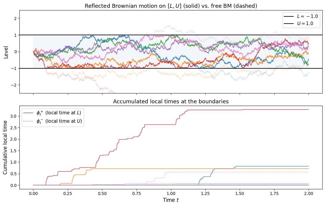
In the upper panel, the solid curves never leave the blue band $[L, U]$, while the dashed free Brownian motions regularly escape. In the lower panel, $\phi^+_t$ (solid lines) grows in steps whenever $X_t$ touches $L$, and $\phi^-_t$ (dotted lines) grows when $X_t$ touches $U$. Both are flat while the process is in the interior — the hallmark of a singular process.

Figure 2 — Local time in action

To see local time in action more clearly, we isolate one path and mark every timestep at which the process touches a boundary.

k = 2  # pick one path for the zoom

tol = 1e-9
hits_L = np.where(np.abs(X[:, k] - L) < tol)[0]
hits_U = np.where(np.abs(X[:, k] - U) < tol)[0]

fig, axes = plt.subplots(3, 1, figsize=(11, 9), sharex=True)

# --- Path ---
ax0 = axes[0]
ax0.plot(t, X[:, k], lw=1.4, color='steelblue', label='$X_t$')
ax0.plot(t, W[:, k], lw=0.9, color='steelblue', alpha=0.3, ls='--', label='$W_t$ (free BM)')
ax0.axhline(L, color='tomato',   lw=1.5, label=f'$L = {L}$')
ax0.axhline(U, color='seagreen', lw=1.5, label=f'$U = {U}$')
ax0.fill_between(t, L, U, alpha=0.07, color='steelblue')

# mark boundary hits
if len(hits_L):
    ax0.scatter(t[hits_L], X[hits_L, k], s=6, color='tomato',   zorder=5)
if len(hits_U):
    ax0.scatter(t[hits_U], X[hits_U, k], s=6, color='seagreen', zorder=5)

ax0.set_ylabel('Level', fontsize=12)
ax0.legend(fontsize=10, ncol=4)
ax0.set_title('Single path — process, free BM, and boundary touches', fontsize=13)

# --- phi_L ---
ax1 = axes[1]
ax1.plot(t, phi_L[:, k], color='tomato', lw=1.4)
ax1.set_ylabel(r'$\phi^+_t$ (cumul. push at $L$)', fontsize=12)
ax1.set_title('Local time at $L$: grows only when $X_t = L$', fontsize=13)

# shade intervals where X == L
in_L = (np.abs(X[:, k] - L) < tol).astype(float)
ax1.fill_between(t, 0, phi_L[:, k].max() * in_L,
                 alpha=0.25, color='tomato', label='$X_t = L$')
ax1.legend(fontsize=10)

# --- phi_U ---
ax2 = axes[2]
ax2.plot(t, phi_U[:, k], color='seagreen', lw=1.4)
ax2.set_ylabel(r'$\phi^-_t$ (cumul. push at $U$)', fontsize=12)
ax2.set_title('Local time at $U$: grows only when $X_t = U$', fontsize=13)
ax2.set_xlabel('Time $t$', fontsize=12)

in_U = (np.abs(X[:, k] - U) < tol).astype(float)
ax2.fill_between(t, 0, phi_U[:, k].max() * in_U,
                 alpha=0.25, color='seagreen', label='$X_t = U$')
ax2.legend(fontsize=10)

plt.tight_layout()
plt.savefig('single_path_local_time.png', dpi=150, bbox_inches='tight')
plt.show()

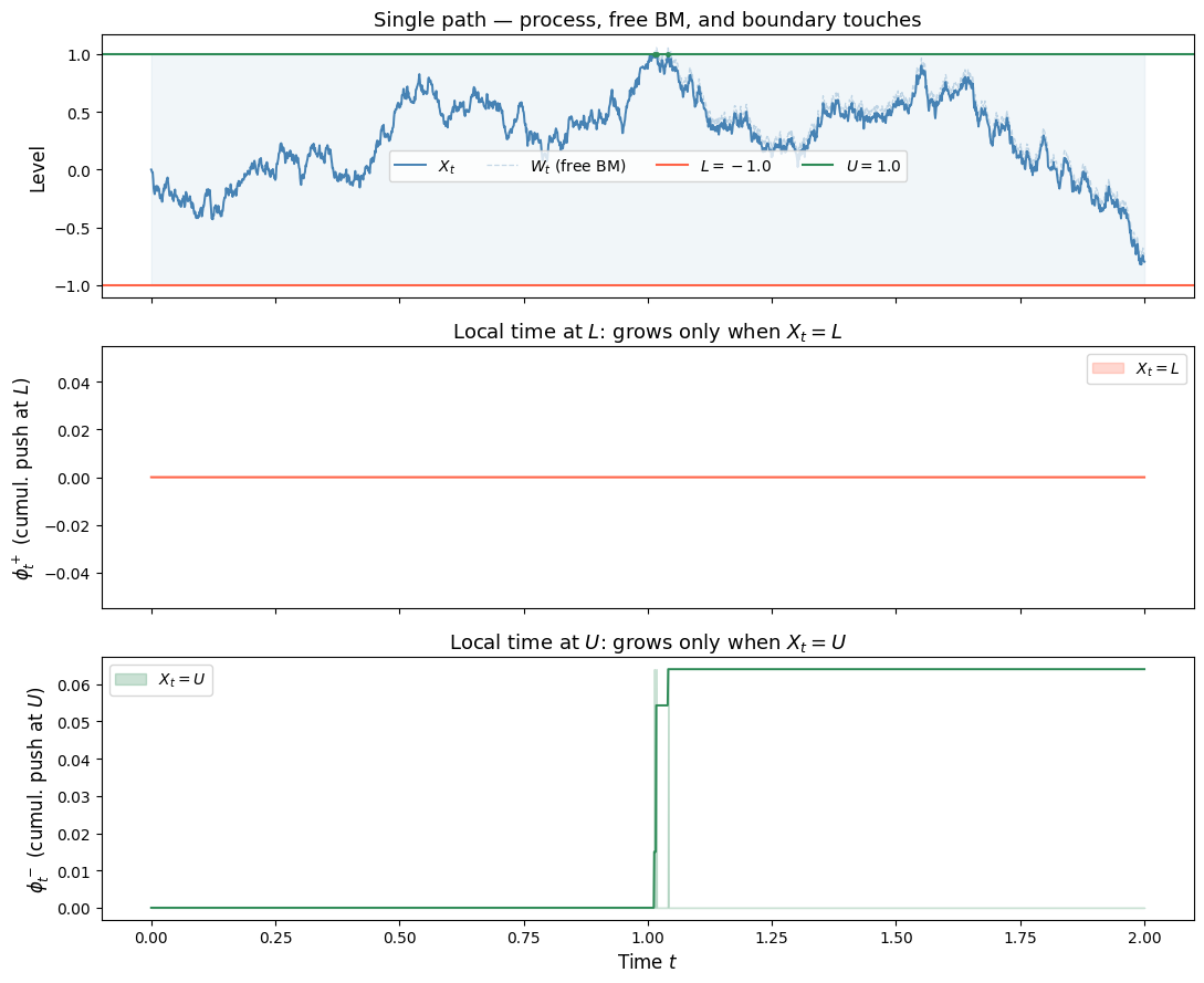
The top panel shows $X_t$ (solid) contained within the band while the free Brownian motion (dashed, faint) wanders freely; red dots mark touches of $L$, green dots mark touches of $U$. The middle and bottom panels reveal the singular structure of local time directly: $\phi^+_t$ is a staircase that steps only within the red-shaded intervals where $X_t = L$, and is perfectly flat everywhere else. $\phi^-_t$ behaves identically at $U$.

Figure 3 — Stationary distribution

A theoretical consequence of the Fokker-Planck analysis is that the long-run stationary distribution of reflected Brownian motion on $[L, U]$ is uniform. We verify this empirically by simulating a large ensemble and examining the marginal distribution at a large time $T$.

_, X_large, _, _, _ = simulate_reflected_bm(T=10.0, N=10_000, n_paths=5_000,
                                             x0=x0, L=L, U=U, seed=99)

fig, ax = plt.subplots(figsize=(7, 4))
ax.hist(X_large[-1, :], bins=60, density=True, color='steelblue', alpha=0.7,
        edgecolor='white', label='Empirical marginal at $T=10$')
ax.axhline(1.0 / (U - L), color='tomato', lw=2, ls='--',
           label=f'Uniform$({L}, {U})$ density = {1/(U-L):.2f}')
ax.set_xlabel('$X_T$', fontsize=12)
ax.set_ylabel('Density', fontsize=12)
ax.set_title('Stationary distribution of reflected BM on $[L, U]$', fontsize=13)
ax.legend(fontsize=11)
plt.tight_layout()

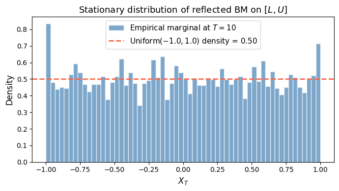
The histogram matches the $\mathrm{Uniform}(L, U)$ density closely, confirming the theoretical prediction. Two remarks are worth making. First, it does not matter where the process starts: the $x_0$-dependence lives entirely in the cosine coefficients, all of which are multiplied by decaying exponentials, so every memory of the initial position is erased on timescale $\tau$. Second, uniformity is a statement about the distribution, not individual paths — any single path continues to bounce around indefinitely, but by ergodicity the fraction of time it spends in any sub-interval $[a, b] \subset [L, U]$ converges to $(b-a)/(U-L)$.

---

4. The Fokker-Planck Equation

The Fokker-Planck (or forward Kolmogorov) equation governs the evolution of the probability density $p(x, t)$ of $X_t$. Since the only forces on $X_t$ are the boundary pushes $d\phi^\pm$, the interior dynamics reduce to the heat equation,

\[\frac{\partial p}{\partial t} = \frac{1}{2}\frac{\partial^2 p}{\partial x^2}, \qquad x \in (L, U),\quad t > 0,\]

with initial condition $p(x, 0) = \delta(x - x_0)$ for a process started at $X_0 = x_0$.

The boundary conditions encode the reflection. In the weak (distributional) form of the equation, the local time terms $d\phi^\pm$ appear as delta-function sources at $x = L$ and $x = U$. Applying the support conditions of the Skorokhod problem — $\phi^+$ active only at $L$, $\phi^-$ only at $U$ — these reduce to zero-flux (Neumann) conditions:

\[\frac{\partial p}{\partial x}\bigg|_{x=L} = 0, \qquad \frac{\partial p}{\partial x}\bigg|_{x=U} = 0.\]

Zero flux means no probability leaks through the walls: everything that reaches a boundary is reflected back. Absorbing walls would instead impose Dirichlet conditions $p(L,t) = p(U,t) = 0$.

Exact solution

The operator $\tfrac{1}{2}\partial_{xx}$ with Neumann boundary conditions on $[L,U]$ has a complete orthogonal basis of cosines. Separation of variables $p(x,t) = \psi(x)\,T(t)$ gives the eigenvalue problem

\[\frac{1}{2}\psi''(x) = -\lambda\,\psi(x), \qquad \psi'(L) = \psi'(U) = 0,\]

whose solutions are $\psi_n(x) = \cos!\left(\frac{n\pi(x-L)}{U-L}\right)$ with eigenvalues $\lambda_n = \frac{n^2\pi^2}{2(U-L)^2}$, for $n = 0, 1, 2, \ldots$ Expanding $p$ in this basis and projecting the initial condition $\delta(x - x_0)$ onto each eigenfunction gives $c_0 = \frac{1}{U-L}$ and $c_n = \frac{2}{U-L}\cos!\left(\frac{n\pi(x_0-L)}{U-L}\right)$ for $n \geq 1$. The exact solution is therefore

\[\boxed{ p(x,t) = \frac{1}{U-L} + \frac{2}{U-L}\sum_{n=1}^{\infty} \cos\!\left(\frac{n\pi(x_0-L)}{U-L}\right) \cos\!\left(\frac{n\pi(x-L)}{U-L}\right) e^{-\frac{n^2\pi^2 t}{2(U-L)^2}} }\]

Three checks confirm the result: at $t = 0$ the cosine series reconstructs $\delta(x - x_0)$; as $t \to \infty$ all $n \geq 1$ terms vanish, leaving the uniform density $\frac{1}{U-L}$; and $\sin(0) = \sin(n\pi) = 0$ so the Neumann conditions are satisfied at both endpoints.

Relaxation timescale

The slowest-decaying mode has $n = 1$, and its decay rate defines the equilibration timescale

\[\tau = \frac{1}{\lambda_1} = \frac{2(U-L)^2}{\pi^2}.\]

The process takes longer to forget its starting point the wider the band — quadratically so. For $L = -1$, $U = 1$ this gives $\tau = 8/\pi^2 \approx 0.81$.

def fokker_planck_exact(x, t, x0, L, U, n_terms=60):
    """Exact solution of the Fokker-Planck equation for reflected BM on [L, U].

    x, t can be scalars or arrays of any broadcastable shape.
    """
    ell = U - L
    x = np.asarray(x, dtype=float)
    t = np.asarray(t, dtype=float)
    shape = np.broadcast_shapes(x.shape, t.shape)
    xf = np.broadcast_to(x, shape).ravel()   # (M,)
    tf = np.broadcast_to(t, shape).ravel()   # (M,)

    kn = np.arange(1, n_terms + 1) * np.pi / ell  # (n_terms,)
    cos_x0 = np.cos(kn * (x0 - L))                 # (n_terms,)

    series = np.sum(
        cos_x0[:, None]
        * np.cos(kn[:, None] * (xf[None, :] - L))
        * np.exp(-(kn[:, None] ** 2 / 2.0) * tf[None, :]),
        axis=0,
    )                                               # (M,)

    return (1.0 / ell + (2.0 / ell) * series).reshape(shape)

Figure 4 — Surface plot of the exact Fokker-Planck solution

We plot $p(x,t)$ as a surface over the $(t, x)$ plane. The density starts as a spike at $x_0$ and spreads out, becoming uniform as $t \gg \tau$.

from mpl_toolkits.mplot3d import Axes3D  # noqa: F401

# Grid — avoid t=0 (delta singularity); start just after
t_grid = np.linspace(0.02, 4.0, 200)
x_grid = np.linspace(L, U, 200)
TT, XX = np.meshgrid(t_grid, x_grid)   # both (200, 200), x varies along axis 0

# p has the same shape as TT and XX
P = fokker_planck_exact(XX, TT, x0=x0, L=L, U=U, n_terms=80)

fig = plt.figure(figsize=(12, 6))

# ── 3-D surface ──────────────────────────────────────────────────────────────
ax3d = fig.add_subplot(121, projection='3d')
surf = ax3d.plot_surface(TT, XX, P, cmap='viridis', linewidth=0,
                         antialiased=True, alpha=0.92)
fig.colorbar(surf, ax=ax3d, shrink=0.5, pad=0.08, label='$p(x,t)$')

# stationary density plane
p_inf = 1.0 / (U - L)
ax3d.plot_surface(TT, XX, np.full_like(P, p_inf),
                  alpha=0.15, color='tomato')

ax3d.set_xlabel('Time $t$', labelpad=8)
ax3d.set_ylabel('$x$', labelpad=6)
ax3d.set_zlabel('$p(x,t)$', labelpad=6)
ax3d.set_title('Exact Fokker-Planck density\n(red plane = uniform stationary)', fontsize=11)
ax3d.view_init(elev=28, azim=-55)

# ── Selected time slices ──────────────────────────────────────────────────────
ax2d = fig.add_subplot(122)
tau_relax = 2.0 * (U - L)**2 / np.pi**2
slice_times = [0.05, 0.2, tau_relax, 2 * tau_relax, 4 * tau_relax]
slice_labels = [f'$t = {tv:.2f}$' for tv in slice_times]
slice_labels[-3] = f'$t = \\tau \\approx {tau_relax:.2f}$'

cmap_slices = plt.cm.plasma(np.linspace(0.1, 0.9, len(slice_times)))
x_fine = np.linspace(L, U, 500)

for tv, label, col in zip(slice_times, slice_labels, cmap_slices):
    p_slice = fokker_planck_exact(x_fine, np.full_like(x_fine, tv),
                                   x0=x0, L=L, U=U, n_terms=80)
    ax2d.plot(x_fine, p_slice, lw=1.8, color=col, label=label)

ax2d.axhline(p_inf, color='tomato', lw=1.5, ls='--', label=r'$p_\infty = 1/(U{-}L)$')
ax2d.axvline(x0, color='k', lw=1.0, ls=':', alpha=0.5, label=f'$x_0 = {x0}$')
ax2d.set_xlabel('$x$', fontsize=12)
ax2d.set_ylabel('$p(x,t)$', fontsize=12)
ax2d.set_title('Time slices of the exact density', fontsize=12)
ax2d.legend(fontsize=9, loc='upper right')
ax2d.set_xlim(L, U)

plt.tight_layout()

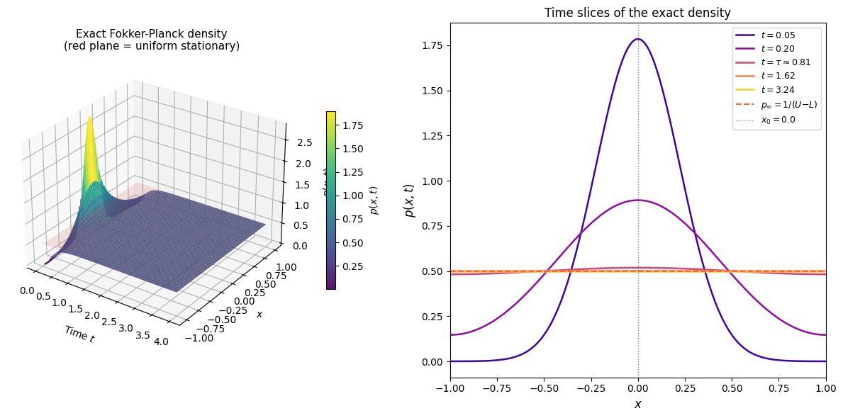
In the left panel, the density starts as a near-spike at $x_0 = 0$ and flattens monotonically toward the red stationary plane $p_\infty = \frac{1}{U-L} = 0.5$. The right panel shows this evolution through time slices: the density is sharply peaked at early times, close to uniform by $t = \tau \approx 0.81$, and virtually indistinguishable from $p_\infty$ by $t = 4\tau$. Since $x_0 = 0$ is the midpoint of $[-1, 1]$, only the odd cosine modes ($n = 1, 3, 5, \ldots$ in the shifted coordinates) are excited, so the density remains symmetric about $x = 0$ for all time.