In the field of financial mathematics, the implied volatility surface is a very usefyul tool with a prominent place for traders and market makers of financial derivatives. In this post we consider the Surface SVI, or SSVI, model for such surface. This model, introduced in 2012 by Gatheral and Jacquier, is built on top of the popular stochastic volatility inspired, or SVI, parametrization of the implied volatility smile, introduced by Gatheral in 2004.
The SSVI model describes the implied volatility surface indirectly by modeling the total implied variance as function $w(y, t)$ such that
\[w(y, t) = \sigma(y, t)^2 t,\]where $t$ is the expiry time t of the option in fractions of the year $y = \log\frac{K}{F(t)}$ the logmoneyness, with $K$ is the strike of the vanilla option and $F(t)$ the value of the forward at time $t$, and $\sigma(t, y)$ the implied volatility at $(y, t)$.
The model is composed by two parts. The first component is the at-the-money total implied variance
\[\psi(t) = \sigma(0, t)^2 t\]for a function $\psi(t)$ that is at least $C^1(\mathbb{R}^+)$ such that
\[\lim_{t\rightarrow 0} \psi(t) = 0.\]Then, given a smooth function $\varphi: \mathbb{R}^+ \rightarrow \mathbb{R}^+$ such that the limit
\[\lim_{\theta\rightarrow 0} \theta \varphi(\theta)\]exists, the SSVI parametrization is given by the formula
\[w(y, t) = \frac{\theta}{2} \left( 1 + \rho \varphi(\theta) y + \sqrt{ \left( \varphi(\theta)y + \rho \right)^2 + (1 - \rho^2) } \right)\]where $\varphi = \psi(t)$, $-1 < \rho < 1$ a real constant. It can be shown that such surface is free of calendar arbitrage if and only if
\[\begin{aligned} &\frac{\partial}{\partial t}\psi(t) \ge 0\quad \forall t \ge 0 \\ % &0 \le \frac{\partial}{\partial \theta}(\theta \varphi(\theta)) \le \frac{1}{\rho^2} \left(1 + \sqrt{1 - \rho^2}\right)\varphi(\theta), \end{aligned}\]and that it is free of butterly arbitrage if and only if
\[\begin{aligned} \theta \varphi(\theta)(1 + |\rho|) & < 4 \\ % \theta \varphi^2(\theta)(1 + |\rho|) & < 4. \end{aligned}\]Some possible choices for $\varphi$ have been presented in the original SSVI paper; here we will use the power-law representation
\[\varphi(\theta) = \eta \theta^{-\lambda}.\]Since $\varphi(\theta) > 0$, clearly $\eta > 0$. From the no-arbitrage conditions above we get
\[\begin{aligned} 0 & \le \eta < \min\left( \frac{4 \theta_M^{\lambda - 1}}{1 + |\rho|}, \frac{2 \theta_M^{\lambda - 1/2}}{\sqrt{1 + |\rho|}}, \right) \\ 0 & \le \lambda \le \frac{1}{2}. \end{aligned}\]from dataclasses import dataclass
import matplotlib.pylab as plt
import numpy as np
import pandas as pd
from scipy.interpolate import interp1d, PchipInterpolator
from scipy.optimize import least_squares
from scipy.stats import norm
Φ = norm.cdf
Φ_inv = norm.ppf
def get_strike(F, T, df, σ, delta, is_call):
    ω = 1 if is_call else -1
    x = -ω * σ * np.sqrt(T) * Φ_inv(abs(delta) / df) + 0.5 * σ**2 * T
    return F * np.exp(x)
The market conditions below are taken from Antonio Castagna book FX Options and Smile Risk.
S_0 = 1.5184
data = pd.read_csv('./EURUSD.csv', sep='\t')
data = data.set_index('Tenor')
data
| T | df_r | df_q | σ_10_DP | σ_15_DP | σ_20_DP | σ_25_DP | σ_35_DP | σ_ATM | σ_35_DC | σ_25_DC | σ_20_DC | σ_15_DC | σ_10_DC | |
|---|---|---|---|---|---|---|---|---|---|---|---|---|---|---|
| Tenor | ||||||||||||||
| 1W | 0.019231 | 0.999387 | 0.999218 | 0.1146 | 0.1125 | 0.1113 | 0.1106 | 0.1098 | 0.1100 | 0.1114 | 0.1135 | 0.1150 | 0.1172 | 0.1203 |
| 2W | 0.038462 | 0.998779 | 0.998429 | 0.1095 | 0.1072 | 0.1058 | 0.1050 | 0.1041 | 0.1040 | 0.1052 | 0.1071 | 0.1085 | 0.1105 | 0.1136 |
| 1M | 0.083333 | 0.997132 | 0.996257 | 0.1051 | 0.1023 | 0.1005 | 0.0993 | 0.0978 | 0.0970 | 0.0975 | 0.0988 | 0.0999 | 0.1015 | 0.1041 |
| 2M | 0.166667 | 0.994686 | 0.992191 | 0.1068 | 0.1035 | 0.1013 | 0.0997 | 0.0977 | 0.0965 | 0.0966 | 0.0977 | 0.0987 | 0.1003 | 0.1029 |
| 3M | 0.250000 | 0.992006 | 0.988242 | 0.1077 | 0.1039 | 0.1012 | 0.0993 | 0.0968 | 0.0953 | 0.0952 | 0.0963 | 0.0973 | 0.0990 | 0.1019 |
| 6M | 0.500000 | 0.985281 | 0.977018 | 0.1100 | 0.1049 | 0.1012 | 0.0986 | 0.0953 | 0.0933 | 0.0932 | 0.0946 | 0.0962 | 0.0984 | 0.1023 |
| 9M | 0.750000 | 0.975910 | 0.966284 | 0.1112 | 0.1055 | 0.1013 | 0.0983 | 0.0947 | 0.0925 | 0.0924 | 0.0939 | 0.0956 | 0.0981 | 0.1025 |
| 1Y | 1.000000 | 0.970856 | 0.956071 | 0.1117 | 0.1056 | 0.1011 | 0.0980 | 0.0941 | 0.0918 | 0.0917 | 0.0932 | 0.0951 | 0.0978 | 0.1026 |
| 2Y | 2.000000 | 0.949348 | 0.927723 | 0.1081 | 0.1072 | 0.0980 | 0.0950 | 0.0913 | 0.0895 | 0.0890 | 0.0902 | 0.0919 | 0.0943 | 0.0987 |
| 5Y | 5.000000 | 0.840130 | 0.824089 | 0.1145 | 0.1052 | 0.0987 | 0.0945 | 0.0890 | 0.0890 | 0.0881 | 0.0897 | 0.0923 | 0.0964 | 0.1041 |
data['r'] = -np.log(data['df_r']) / data['T']
data['q'] = -np.log(data['df_q']) / data['T']
data['F'] = S_0 * data['df_q'] / data['df_r']
data['K_ATM'] = data['F'] * np.exp(0.5 * data['σ_ATM']**2 * data['T'])
for Δ in [10, 15, 20, 25, 35]:
    data[f'K_{Δ}_DP'] = get_strike(data['F'], data['T'], data['df_q'], data[f'σ_{Δ}_DP'], -Δ / 100, False)
    data[f'K_{Δ}_DC'] = get_strike(data['F'], data['T'], data['df_q'], data[f'σ_{Δ}_DC'], Δ / 100, True)
data.loc['2Y']['K_ATM'] = data.loc['2Y']['F']
data.loc['5Y']['K_ATM'] = data.loc['5Y']['F']
data['Y_ATM'] = np.log(data['K_ATM'] / data['F'])
for Δ in [10, 15, 20, 25, 35]:
    data[f'Y_{Δ}_DP'] = np.log(data[f'K_{Δ}_DP'] / data['F'])
    data[f'Y_{Δ}_DC'] = np.log(data[f'K_{Δ}_DC'] / data['F'])
data['V_ATM'] = data['σ_ATM']**2 * data['T']
for Δ in [10, 15, 20, 25, 35]:
    data[f'V_{Δ}_DP'] = data[f'σ_{Δ}_DP']**2 * data['T']
    data[f'V_{Δ}_DC'] = data[f'σ_{Δ}_DC']**2 * data['T']
@dataclass
class Smile:
    tenor: str
    T: str   # tenors
    K: list  # strikes
    Y: list  # log-moneyness
    V: list  # implied variance

    def __post_init__(self):
        self.interp = interp1d(self.Y, self.V, kind='cubic')

    # input is logmoneyness
    def get_vol(self, y):
        return float(self.interp(y))
for tenor, slice in data.iterrows():
y_slice = slice[[
'Y_10_DP', 'Y_15_DP', 'Y_20_DP', 'Y_25_DP', 'Y_35_DP',
'Y_ATM',
'Y_35_DC', 'Y_25_DC', 'Y_20_DC', 'Y_15_DC', 'Y_10_DC',
]]
σ_slice = slice[[
'σ_10_DP', 'σ_15_DP', 'σ_20_DP', 'σ_25_DP', 'σ_35_DP',
'σ_ATM',
'σ_35_DC', 'σ_25_DC', 'σ_20_DC', 'σ_15_DC', 'σ_10_DC',
]]
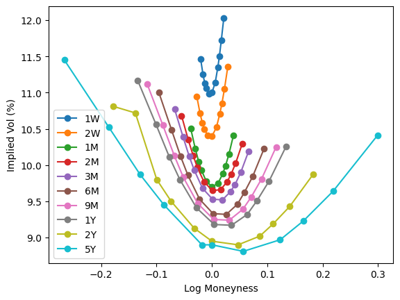
plt.plot(y_slice, 100 * σ_slice, 'o-', label=tenor)
plt.legend()
plt.xlabel('Log Moneyness')
plt.ylabel('Implied Vol (%)');
smiles = []

for tenor, slice in data.iterrows():
    K_slice = slice[[
        'K_10_DP', 'K_15_DP', 'K_20_DP', 'K_25_DP', 'K_35_DP',
        'K_ATM',
        'K_35_DC', 'K_25_DC', 'K_20_DC', 'K_15_DC', 'K_10_DC',
    ]]

    Y_slice = slice[[
        'Y_10_DP', 'Y_15_DP', 'Y_20_DP', 'Y_25_DP', 'Y_35_DP',
        'Y_ATM',
        'Y_35_DC', 'Y_25_DC', 'Y_20_DC', 'Y_15_DC', 'Y_10_DC',
    ]]

    V_slice = slice[[
        'V_10_DP', 'V_15_DP', 'V_20_DP', 'V_25_DP', 'V_35_DP',
        'V_ATM',
        'V_35_DC', 'V_25_DC', 'V_20_DC', 'V_15_DC', 'V_10_DC',
    ]]

    smiles.append(Smile(tenor, slice['T'], K_slice, Y_slice, V_slice))
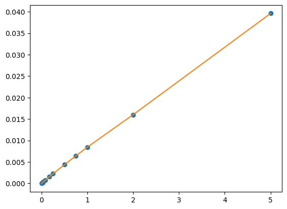
For the function $\psi$, we use the scipys piecewise cubic Hermite interpolating polynomial, which preserves monotonicity in the interpolation data and does not overshoot if the data is not smooth. We are also guaranteed to have continuous first derivatives, which are needed to compute the local volatilities from the surface as we will see below.
t_all, V_ATM_all = [0], [0]  # variance at t=0 must be 0

for smile in smiles:
    t_all.append(smile.T)
    V_ATM_all.append(smile.get_vol(0.0))

ψ = PchipInterpolator(t_all, V_ATM_all)

plt.plot(t_all, V_ATM_all, 'o')
plt.plot(t_all, ψ(t_all))
[<matplotlib.lines.Line2D at 0x23ffebaf8b0>]
T_all, Y_all, V_all = [], [], []
for smile in smiles:
    T_all.append(smile.T)
    Y_all.append(smile.Y.values)
    V_all.append(smile.V.values)
def compute_w(Y, T, η, λ, ρ):
    θ = ψ(T)
    φ = η * np.power(θ, -λ)
    return θ / 2 * (1 + ρ * φ * Y + np.sqrt((φ * Y + ρ)**2 + (1 - ρ**2)))
The fitting procedure is quite standard, minimizing the square of the difference between the market implied volatility and the SSVI one. (It is also possible to compare prices directly, which is more accurate in low delta regions.) A penalty term is added to take into account the nonlinear upper bound on $\eta$, while the other bounds are directly given in input to the least_square() method.
def f(x):
    η = x[0]
    λ = x[1]
    ρ = x[2]
    retval = []
    θ_max = ψ(T_all[-1])
    η_max = min(4 * np.power(θ_max, λ - 1) / (1 + abs(ρ)), 2 * np.power(θ_max, λ - 0.5) / np.sqrt(1 + abs(ρ)))
    penalty = 1e-4 * (η - η_max)**2 if η > η_max else 0
    for T, Y_smile, V_smile in zip(T_all, Y_all, V_all):
        for X, V in zip(Y_smile, V_smile):
            V_hat = compute_w(X, T, η, λ, ρ)
            retval.append((V_hat - V)**2 + penalty)
    return retval

res = least_squares(f, [0.2, 0.25, 0.0], bounds=([0, 0, -1], [np.inf, 0.5, 1]))
assert res.success
η, λ, ρ = res.x
print(f'η = {η:.4f}, λ = {λ:.4f}, ρ = {ρ:.4f}')
η = 1.5830, λ = 0.3818, ρ = -0.1332
The fit is very fast. To assess the quality, we plot implied volatlity from the market and compare them with the SSVI prediction for all the maturities we have used.
fig, axes = plt.subplots(figsize=(8, 15), nrows=5, ncols=2)
axes = axes.flatten()
for ax, smile in zip(axes, smiles):
    V_hat_all = []
    for Y, V in zip(smile.Y, smile.V):
        V_hat_all.append(compute_w(Y, smile.T, η, λ, ρ))

    ax.plot(smile.Y, 100 * np.sqrt(smile.V / smile.T), '-o', label='Market')
    ax.plot(smile.Y, 100 * np.sqrt(V_hat_all / smile.T), '-', label='SSVI')
    ax.set_xlabel('Logmoneyness')
    ax.set_ylabel('Implied Volatility (%)')
    ax.set_title(f'T = {smile.tenor}')
    ax.legend()

fig.tight_layout()
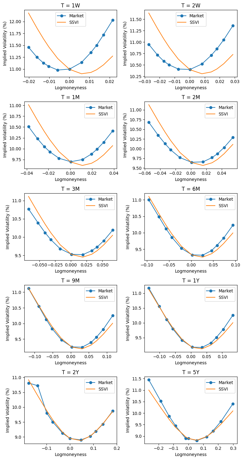
Looking at the plot, we realize that the quality of the fit is quite bad for short maturities, while it is good for medium and long maturities. This is expected for the considered market conditions – begin $\rho$ constant, it can’t change over time as it should to fit the data. This means that the model is not very flexible; more flexible models like Extended SSVI may have helped.
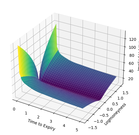
We now proceed to use the volatility surface as part of the local volatility model
\[\begin{aligned} dS(t) / S(t) & = (r - q) dt + \sigma_{loc}(S(t), t) dW(t) \\ S(0) & = S_0. \end{aligned}\]Given a surface $w(y, t)$ describing the toal implied variance, it is well-known that the local volatility $\sigma_{loc}(y, t)$, as function of logmoneyness and time, is given by the formula
\[\sigma_{loc}^2 = \frac{ \frac{\partial w}{\partial t} }{ 1 - \frac{\partial w}{\partial y} \frac{1}{w}\left( y + \frac{1}{4} \frac{\partial w}{\partial y} \left( 1 + \frac{1}{4} w - \frac{y^2}{w} \right) \right) + \frac{1}{2}\frac{\partial^2 w}{\partial y^2} }.\]What we will do is to compute the implied volatility of options priced with the local volatility model and compare them with the ones provided by the SSVI formula.
def get_local_vol(Y, T, η, λ, ρ, ΔT, ΔY):
    T = max(T, 1.1 * ΔT)
    w = compute_w(Y, T, η, λ, ρ)
    w_plus_ΔT = compute_w(Y, T + ΔT, η, λ, ρ)
    w_minus_ΔT = compute_w(Y, T - ΔT, η, λ, ρ)
    num = (w_plus_ΔT - w_minus_ΔT) / 2 / ΔT
    w_plus_ΔY = compute_w(Y + ΔY, T, η, λ, ρ)
    w_minus_ΔY = compute_w(Y - ΔY, T, η, λ, ρ)
    w_prime = (w_plus_ΔY - w_minus_ΔY) / 2 / ΔY
    w_second = (w_plus_ΔY - 2 * w + w_minus_ΔY) / ΔY**2
    den = 1 - w_prime / w * (Y + 1 / 4 * w_prime * (1 + 1 / 4 * w - Y**2 / w)) \
        + 1 / 2 * w_second
    return np.sqrt(num / den)
First, we plot the local volatility $\sigma_{loc}(y, t)$.
Y_all = np.linspace(-1.5, 1.5, 101)
T_all = np.linspace(1 / 256, 5, 101)
ZZ = []
for T in T_all:
    Z_all = get_local_vol(Y_all, T, η, λ, ρ, 1e-5, 1e-5)
    ZZ.append(Z_all * 100)
XX, TT = np.meshgrid(Y_all, T_all)
ZZ = np.array(ZZ)
fig = plt.figure()
ax = plt.axes(projection='3d')
ax.plot_surface(TT, XX, ZZ, cmap='viridis')
ax.set_xlabel('Time to Expiry')
ax.set_ylabel('Logmoneyness')
ax.set_zlabel('Implied Vol (%)')
fig.tight_layout()
class ZeroRate:
    def __init__(self, T, rates):
        self.T = T
        accumulated = T * rates
        self.rates = np.concatenate((rates[:1], np.diff(accumulated) / np.diff(T)))

    def __call__(self, t):
        index = np.searchsorted(self.T, t, side='left')
        if index > len(self.T):
            index = -1
        return self.rates[index]
r_curve = ZeroRate(data['T'], data['r'])
q_curve = ZeroRate(data['T'], data['q'])
schedule = [0.0]
t = 0
for tenor in data['T']:
    # one step per day
    max_Δt = 1 / 256
    if tenor < 1.01 / 12:
        # a bit finer at the beginning
        max_Δt /= 4
    num_steps = int(np.ceil((tenor - t) / max_Δt)) + 1
    schedule += np.linspace(t, tenor, num_steps).tolist()[1:]
    t = tenor
print(f"Using {len(schedule)} total points in time.")
Using 1347 total points in time.
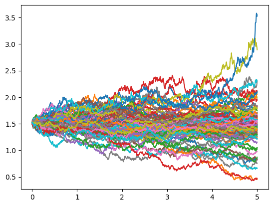
Now we have all the ingredients for a simple Monte Carlo solver.
num_paths = 40_000

paths = [np.ones((num_paths,)) * S_0]
X = np.log(paths[0])
num_steps = len(schedule) - 1
W = norm.rvs(size=(num_steps, num_paths))
log_F = np.log(S_0)
for i in range(num_steps):
    t = schedule[i]
    Δt = schedule[i + 1] - t
    sqrt_Δt = np.sqrt(Δt)
    r, q = r_curve(t), q_curve(t)
    Y = X - log_F
    σ = get_local_vol(Y, t, η, λ, ρ, 1e-5, 1e-5)
    X = X + (r - q - 0.5 * σ**2) * Δt + σ * sqrt_Δt * W[i, :]
    paths.append(np.exp(X))
    log_F += (r - q) * Δt

paths = np.vstack(paths)
Visualize a few paths to get an idea of how they look.
for i in range(100):
    plt.plot(schedule, paths[:, i])
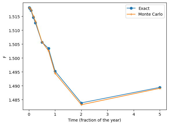
We can check that our Monte Carlo matches the forward value reasonably well.
T_all, F_all, F_mc_all = [], [], []
for tenor in data.index:
    T = data.loc[tenor]['T']
    T_all.append(T)
    F_all.append(data.loc[tenor]['F'])
    index = schedule.index(T)
    F_mc_all.append(paths[index, :].mean())
plt.plot(T_all, F_all, '-o', label='Exact')
plt.plot(T_all, F_mc_all, '-+', label='Monte Carlo')
plt.xlabel('Time (fraction of the year)')
plt.ylabel('F')
plt.legend()
<matplotlib.legend.Legend at 0x23fff671720>
We are ready to verify the correctness of our local volatility formula. We do this by looping over all tenors in the original surface and computing, for several strikes from the 10 delta put strike to the 10 delta call strike, the implied volatility corresponding to the price generated by the Monte Carlo solver. For simplicity we use straddles, so a call and a put with the same strike, to avoid looking for the put and call flag.
def black_scholes_price(F, K, T, df, σ):
    assert T > 0.0
    # a call and a put with the same strike
    d_plus = (np.log(F / K) + 0.5 * σ**2 * T) / σ / np.sqrt(T)
    d_minus = d_plus - σ * np.sqrt(T)
    retval = 0
    for ω in [-1, 1]:
        retval += ω * df * (F * Φ(ω * d_plus) - K * Φ(ω * d_minus))
    return retval
def compute_implied_vol(F, K, T, df, target_price):
    from scipy.optimize import root_scalar
    try:
        f = lambda σ_implied: black_scholes_price(F, K, T, df, σ_implied) - target_price
        result = root_scalar(f, method='brentq', bracket=(1e-4, 1.0))
        return result.root if result.converged else np.nan
    except:
        return np.nan
def plot_mc_results(tenor, ax):
    K_min, K_max = data.loc[tenor]['K_10_DP'], data.loc[tenor]['K_10_DC']
    K_all = np.linspace(K_min, K_max, 101)
    σ_mc_up_all, σ_mc_down_all, σ_exact_all = [], [], []
    T = data.loc[tenor]['T']
    F = data.loc[tenor]['F']
    df = data.loc[tenor]['df_r']
    index = schedule.index(T)

    for K in K_all:
        Π = df * abs(paths[index, :] - K)
        target_price = Π.mean()
        target_std_dev = Π.std() / np.sqrt(num_paths)
        σ_mc_down_all.append(compute_implied_vol(F, K, T, df, target_price - 1.96 * target_std_dev))
        σ_mc_up_all.append(compute_implied_vol(F, K, T, df, target_price + 1.96 * target_std_dev))
        Y = np.log(K / F)
        σ_exact_all.append(np.sqrt(compute_w(Y, T, η, λ, ρ) / T))

    ax.fill_between(K_all, σ_mc_down_all, σ_mc_up_all, alpha=0.5, color='salmon', label='95% Confidence Interval')
    ax.plot(K_all, σ_exact_all, label='SSVI')
    ax.set_title(tenor)
    ax.legend()
fig, axes = plt.subplots(figsize=(8, 15), nrows=5, ncols=2, sharey=True)
axes = axes.flatten()
for tenor, ax in zip(data.index, axes):
    plot_mc_results(tenor, ax)
fig.tight_layout()
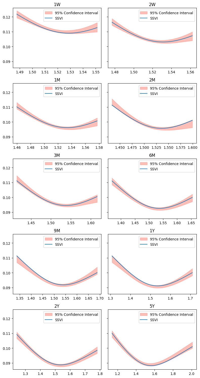
Results are in good agreement, and could be improved by either increasing the resolution of the time grid (so adding more points to the schedule vector) or by increasing the number of paths.