In this article we will look at stacking, or stacked generalization, which is a sophisticated ensemble method designed to leverage on the collective strengths of multiple models.
Different machine learning models have different strenghts and often complementary. In some cases there is a clear winner; often, there isn’t. Stacking allows us to use many models; its efficacy lies in its ability to mitigate the weaknesses of any single model while amplifying their collective strengths. By leveraging the complementary nature of different algorithms, stacking can achieve superior generalization and predictive accuracy, particularly in complex or high-dimensional datasets.
Stacking represents a paradigm shift from traditional ensemble techniques, such as bagging or boosting. Rather than aggregating predictions through averaging or weighted voting, stacking introduces a hierarchical approach: a meta-model is trained to optimally combine the outputs of diverse base models. This meta-model, often a linear regressor or classifier, learns to correct errors and emphasize the most reliable predictions, resulting in a final model that frequently surpasses the performance of its individual components.
A mathematical description of stacking is as follows.
Let $\mathcal{M} = {m_1, m_2, \dots, m_k}$ be a set of $k$ base models, where each model $m_i$ is trained on the $n$ samples each with $p$ input features $\mathbf{X} \in \mathbb{R}^{n \times p}$ and produces predictions $\hat{y}_i$ for the target variable $y \in \mathbb{R}^n$. For each base model $m_i$,
\[\hat{y}_i = m_i(\mathbf{X}).\]The predictions of the base models $\hat{y}_1, \hat{y}_2, \dots, \hat{y}_k$ are combined into a new feature matrix $\mathbf{Z} \in \mathbb{R}^{n \times k}$, where each column represents the predictions of one base model:
\[\mathbf{Z} = [\hat{y}_1, \hat{y}_2, \dots, \hat{y}_k].\]A meta-model $f$ (typically linear regression, logistic regression, or another machine learning algorithm) is trained on the meta-features $\mathbf{Z}$ to produce the final prediction $y^\hat{y}$y,
\[\hat{y} = f(\mathbf{Z}).\]The two components operate on different levels: the base models provide diversity, the meta model allows generation by learning to weight or combine the base models’ predictions optimally, often outperforming any single base model. This procedure often corrects the errors of the base models and emphasizes their strengths.
We will implement stacking in two ways. First we start build each individual component following the above procedure, which is useful to learn and understand all the steps involved. Then we use scikit-learn’s StackingRegressor class; this class performs all the steps internally and it is very easy to use.
import numpy as np
import pandas as pd
We will use a small dataset and start with classical exploratory data analysis.
from sklearn.datasets import fetch_california_housing
housing = fetch_california_housing(as_frame=True)
print(f"The dataset has {housing.data.shape[0]:,} rows and {housing.data.shape[1]} columns")
print(housing.DESCR)
The dataset has 20,640 rows and 8 columns
.. _california_housing_dataset:

California Housing dataset
--------------------------

**Data Set Characteristics:**

:Number of Instances: 20640

:Number of Attributes: 8 numeric, predictive attributes and the target

:Attribute Information:
    - MedInc        median income in block group
    - HouseAge      median house age in block group
    - AveRooms      average number of rooms per household
    - AveBedrms     average number of bedrooms per household
    - Population    block group population
    - AveOccup      average number of household members
    - Latitude      block group latitude
    - Longitude     block group longitude

:Missing Attribute Values: None

This dataset was obtained from the StatLib repository.
https://www.dcc.fc.up.pt/~ltorgo/Regression/cal_housing.html

The target variable is the median house value for California districts,
expressed in hundreds of thousands of dollars ($100,000).

This dataset was derived from the 1990 U.S. census, using one row per census
block group. A block group is the smallest geographical unit for which the U.S.
Census Bureau publishes sample data (a block group typically has a population
of 600 to 3,000 people).

A household is a group of people residing within a home. Since the average
number of rooms and bedrooms in this dataset are provided per household, these
columns may take surprisingly large values for block groups with few households
and many empty houses, such as vacation resorts.

It can be downloaded/loaded using the
:func:`sklearn.datasets.fetch_california_housing` function.

.. rubric:: References

- Pace, R. Kelley and Ronald Barry, Sparse Spatial Autoregressions,
  Statistics and Probability Letters, 33 (1997) 291-297
df = pd.concat((housing.data, housing.target), axis='columns')
assert df.isnull().sum().sum() == 0
df.sample(5)
| MedInc | HouseAge | AveRooms | AveBedrms | Population | AveOccup | Latitude | Longitude | MedHouseVal | |
|---|---|---|---|---|---|---|---|---|---|
| 13758 | 6.5648 | 32.0 | 7.355844 | 1.020779 | 1033.0 | 2.683117 | 34.03 | -117.15 | 2.372 |
| 13366 | 4.2578 | 36.0 | 5.258824 | 1.117647 | 2886.0 | 33.952941 | 33.94 | -117.63 | 1.833 |
| 11804 | 2.9866 | 45.0 | 5.441281 | 1.128114 | 793.0 | 2.822064 | 38.89 | -121.30 | 0.913 |
| 4589 | 1.6184 | 52.0 | 2.170396 | 1.060241 | 2309.0 | 3.974182 | 34.06 | -118.28 | 2.250 |
| 7682 | 3.1397 | 33.0 | 4.400000 | 0.970149 | 1205.0 | 3.597015 | 33.93 | -118.10 | 1.668 |
All the entries are numerical and there are no missing data.
df.info()
<class 'pandas.core.frame.DataFrame'>
RangeIndex: 20640 entries, 0 to 20639
Data columns (total 9 columns):
 #   Column       Non-Null Count  Dtype
---  ------       --------------  -----
 0   MedInc       20640 non-null  float64
 1   HouseAge     20640 non-null  float64
 2   AveRooms     20640 non-null  float64
 3   AveBedrms    20640 non-null  float64
 4   Population   20640 non-null  float64
 5   AveOccup     20640 non-null  float64
 6   Latitude     20640 non-null  float64
 7   Longitude    20640 non-null  float64
 8   MedHouseVal  20640 non-null  float64
dtypes: float64(9)
memory usage: 1.4 MB
import matplotlib.pylab as plt
import seaborn as sns
plt.figure(figsize=(8,5))
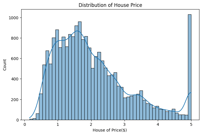
sns.histplot(df.MedHouseVal,bins=50,kde=True)
plt.title("Distribution of House Price")
plt.xlabel("House of Price($) ");
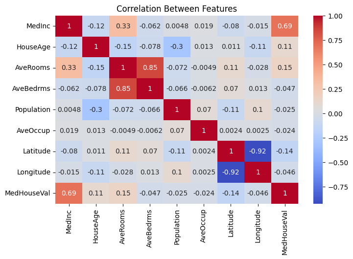
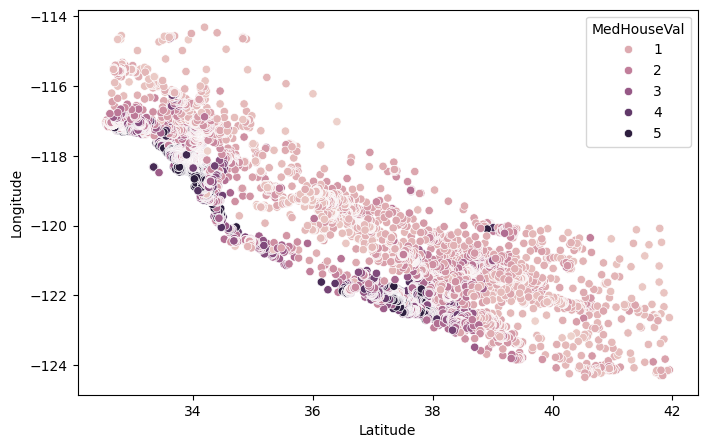
The only feature that is heavily correlated with the target is the median income of the block where the house is located, which simply means that the best predictor of a house price are the prices of neighboring houses. Latitudes and longitudes are highly correlated, as we will see below this is because the coasts roughly are on a line, and coastal areas are more expensive than areas far from the coast.
plt.figure(figsize=(8,5))
sns.heatmap(df.select_dtypes(include='number').corr(),annot=True,cmap='coolwarm')
plt.title("Correlation Between Features");
plt.figure(figsize=(8,5))
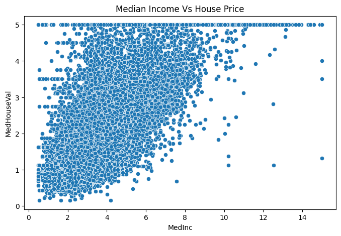
sns.scatterplot(data=df, x='MedInc', y='MedHouseVal')
plt.title("Median Income Vs House Price");
plt.figure(figsize=(20, 5))
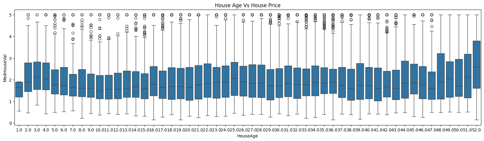
sns.boxplot(data=df, x='HouseAge', y='MedHouseVal')
plt.title("House Age Vs House Price");
plt.figure(figsize=(8,5))
sns.scatterplot(data=df, x='Latitude', y = 'Longitude', hue='MedHouseVal')
<Axes: xlabel='Latitude', ylabel='Longitude'>
We don’t perform any feature engineering, this is a small dataset and we only have a few features.
X = housing.data
y = housing.target.values

# to remove the many entries > 5k
# X = X[y < 5]
# y = y[y < 5]

print(f"\nTarget statistics:")
print(f"  Mean: ${y.mean():.2f} (×100k) = ${y.mean()*100:.0f}k")
print(f"  Median: ${np.median(y):.2f} (×100k) = ${np.median(y) * 100:.0f}k")
print(f"  Std: ${y.std():.2f} (×100k)")
print(f"  Min: ${y.min():.2f} (×100k)")
print(f"  Max: ${y.max():.2f} (×100k)\n")
Target statistics:
  Mean: $2.07 (×100k) = $207k
  Median: $1.80 (×100k) = $180k
  Std: $1.15 (×100k)
  Min: $0.15 (×100k)
  Max: $5.00 (×100k)
from sklearn.preprocessing import StandardScaler
scaler = StandardScaler()
X_scaled = scaler.fit_transform(X)
from sklearn.model_selection import train_test_split, KFold
X_train, X_test, y_train, y_test = train_test_split(X_scaled, y, test_size=0.2, random_state=42)
print(f"# train rows: {len(X_train):,}, # test rows: {len(X_test):,}")
# train rows: 16,512, # test rows: 4,128
In this first phase we use only two regressors: a random forest and a gradient boosting regressor. The meta model, instead, is defined using linear regression.
from sklearn.ensemble import RandomForestRegressor, GradientBoostingRegressor
rf = RandomForestRegressor(n_estimators=100, random_state=42)
gb = GradientBoostingRegressor(n_estimators=100, random_state=42)
When fitting stacking models it is very important to avoid overfitting. Two approaches are widely used: the first one uses $K-$fold to split the training dataset into n_splits components and iterating over the folds. For any of them, we fit a model leaving it out, the we predict on the fold that was left out. After iterating over all the folds, we have the predictions on the entire train dataset. The other approach is to divide the train datasets into two components, fit the model on the first part and predict on the second; the meta model will then be fitted on the second part only. The first approach is more computationally expensive but takes full advantage of the train dataset; the second requires less resources but can be used only for large datasets. Here we follow the first approach.
kf = KFold(n_splits=5, shuffle=True, random_state=42)
rf_oof_pred = np.zeros_like(y_train, dtype=float)
gb_oof_pred = np.zeros_like(y_train, dtype=float)

for train_idx, val_idx in kf.split(X_train):
    X_train_fold, X_val_fold = X_train[train_idx], X_train[val_idx]
    y_train_fold, y_val_fold = y_train[train_idx], y_train[val_idx]

    rf.fit(X_train_fold, y_train_fold)
    gb.fit(X_train_fold, y_train_fold)

    rf_oof_pred[val_idx] = rf.predict(X_val_fold)
    gb_oof_pred[val_idx] = gb.predict(X_val_fold)

X_train_meta = np.column_stack((rf_oof_pred, gb_oof_pred))

from sklearn.linear_model import LinearRegression
meta_model = LinearRegression()
_ = meta_model.fit(X_train_meta, y_train)
The $K-$fold procedure is needed for the meta model; once this is fitted, we recalibrate the base models with the full train dataset.
rf.fit(X_train, y_train)
gb.fit(X_train, y_train);
We are ready to evalute the model:
rf_pred_test = rf.predict(X_test)
gb_pred_test = gb.predict(X_test)
X_test_meta = np.column_stack((rf_pred_test, gb_pred_test))
meta_pred = meta_model.predict(X_test_meta)
from sklearn.metrics import mean_absolute_error, mean_squared_error, r2_score

rf_rmse = np.sqrt(mean_squared_error(y_test, rf_pred_test))
gb_rmse = np.sqrt(mean_squared_error(y_test, gb_pred_test))
meta_rmse = np.sqrt(mean_squared_error(y_test, meta_pred))

print('RMSE:')
print(f"- random forest: {rf_rmse:.3f}")
print(f"- gradient boosting: {gb_rmse:.3f}")
print(f"- stacked model: {meta_rmse:.3f}")

rf_rmse = r2_score(y_test, rf_pred_test)
gb_rmse = r2_score(y_test, gb_pred_test)
meta_rmse = r2_score(y_test, meta_pred)

print('\nR2 score:')
print(f"- random forest: {rf_rmse:.3f}")
print(f"- gradient boosting: {gb_rmse:.3f}")
print(f"- stacked model: {meta_rmse:.3f}")
RMSE:
- random forest: 0.506
- gradient boosting: 0.542
- stacked model: 0.504

R2 score:
- random forest: 0.805
- gradient boosting: 0.776
- stacked model: 0.806
The performance improvement is small but noticeable. Let’s try now with more models and the StackingRegressor class. We keep a linear regressor for the meta model.
from sklearn.ensemble import RandomForestRegressor, GradientBoostingRegressor, StackingRegressor
from sklearn.linear_model import Ridge, Lasso, ElasticNet
from sklearn.svm import SVR
base_models = [
    ('ridge', Ridge()),
    # ('lasso', Lasso()),
    # ('elastic', ElasticNet(alpha=1.0, l1_ratio=0.5)),
    ('rf', RandomForestRegressor(n_estimators=100, random_state=42)),
    ('gb', GradientBoostingRegressor(n_estimators=100, random_state=42)),
    ('svr', SVR(kernel='rbf', C=1.0))
]
meta_model = LinearRegression()
for name, model in base_models:
    model.fit(X_train, y_train)
    y_pred = model.predict(X_test)

    rmse = np.sqrt(mean_squared_error(y_test, y_pred))
    mae = mean_absolute_error(y_test, y_pred)
    r2 = r2_score(y_test, y_pred)

    print(f"{name} model: RMSE = {rmse:.3f}, MAE = {mae:.3f}, R² = {r2:.3f}")
ridge model: RMSE = 0.746, MAE = 0.533, R² = 0.576
rf model: RMSE = 0.506, MAE = 0.328, R² = 0.805
gb model: RMSE = 0.542, MAE = 0.372, R² = 0.776
svr model: RMSE = 0.596, MAE = 0.398, R² = 0.729
stacking_reg = StackingRegressor(
    estimators=base_models,
    final_estimator=meta_model,
    cv=5,
    n_jobs=-1
)

stacking_reg.fit(X_train, y_train)
y_pred_stack = stacking_reg.predict(X_test)

rmse = np.sqrt(mean_squared_error(y_test, y_pred_stack))
mae = mean_absolute_error(y_test, y_pred_stack)
r2 = r2_score(y_test, y_pred_stack)

print(f"Stacking model: RMSE = {rmse:.3f}, MAE = {mae:.3f}, R² = {r2:.3f}")
Stacking model: RMSE = 0.500, MAE = 0.327, R² = 0.809
Here the improvement is a bit larger: while the MAE is as good as the random forest model, the RMSE is smaller and the $R^2$ is higher, showing the effect of stacking.
Some final notes:
- if a single model achieves already a high $R^2$ (say above 0.85), then stacking will likely not help;
- stacking is only useful with multiple, diverse base models, for example trees and neural networks. If you have just one model, focus on improving it directly (e.g., tuning, feature engineering) or use other ensemble methods like bagging or boosting;
- for prediction, stacking requires to load up in memory more models. Memory consumption and evaluation time should be considered when performances are critical.