In this article we will explore stochastic weighted average method. We will use the CoverType dataset. The goal is to predict the forest cover type from cartographic variables only (no remotely sensed data), of which rhere are 7 forest:
Independent variables were derived from data originally obtained from US Geological Survey (USGS) and USFS data. Data is in raw form (not scaled) and contains binary (0 or 1) columns of data for qualitative independent variables (wilderness areas and soil types). The labels represent the dominant species of trees found on a 30m × 30m forest cell, as determinedfrom the US Forest Service (USFS) Region 2 Resource Information System (RIS) data. We will use thew data as provided by the scikit-learn function fetch_covtype().
import matplotlib.pylab as plt
plt.style.use('ggplot')
import numpy as np
import pandas as pd
import seaborn as sns
from sklearn.datasets import fetch_covtype
data = fetch_covtype()
df = pd.concat((
    pd.DataFrame(data.data, columns=data.feature_names),
    pd.DataFrame(data.target - 1, columns=data.target_names)
), axis='columns')
print(f"Dataset contains {df.shape[0]:,} rows and {df.shape[1]:,} columns.")
df.head()
Dataset contains 581,012 rows and 55 columns.
| Elevation | Aspect | Slope | Horizontal_Distance_To_Hydrology | Vertical_Distance_To_Hydrology | Horizontal_Distance_To_Roadways | Hillshade_9am | Hillshade_Noon | Hillshade_3pm | Horizontal_Distance_To_Fire_Points | ... | Soil_Type_31 | Soil_Type_32 | Soil_Type_33 | Soil_Type_34 | Soil_Type_35 | Soil_Type_36 | Soil_Type_37 | Soil_Type_38 | Soil_Type_39 | Cover_Type | |
|---|---|---|---|---|---|---|---|---|---|---|---|---|---|---|---|---|---|---|---|---|---|
| 0 | 2596.0 | 51.0 | 3.0 | 258.0 | 0.0 | 510.0 | 221.0 | 232.0 | 148.0 | 6279.0 | ... | 0.0 | 0.0 | 0.0 | 0.0 | 0.0 | 0.0 | 0.0 | 0.0 | 0.0 | 4 |
| 1 | 2590.0 | 56.0 | 2.0 | 212.0 | -6.0 | 390.0 | 220.0 | 235.0 | 151.0 | 6225.0 | ... | 0.0 | 0.0 | 0.0 | 0.0 | 0.0 | 0.0 | 0.0 | 0.0 | 0.0 | 4 |
| 2 | 2804.0 | 139.0 | 9.0 | 268.0 | 65.0 | 3180.0 | 234.0 | 238.0 | 135.0 | 6121.0 | ... | 0.0 | 0.0 | 0.0 | 0.0 | 0.0 | 0.0 | 0.0 | 0.0 | 0.0 | 1 |
| 3 | 2785.0 | 155.0 | 18.0 | 242.0 | 118.0 | 3090.0 | 238.0 | 238.0 | 122.0 | 6211.0 | ... | 0.0 | 0.0 | 0.0 | 0.0 | 0.0 | 0.0 | 0.0 | 0.0 | 0.0 | 1 |
| 4 | 2595.0 | 45.0 | 2.0 | 153.0 | -1.0 | 391.0 | 220.0 | 234.0 | 150.0 | 6172.0 | ... | 0.0 | 0.0 | 0.0 | 0.0 | 0.0 | 0.0 | 0.0 | 0.0 | 0.0 | 4 |
5 rows × 55 columns
The dataset is of medium size; all entries are valid.
missing_data = df.isnull().sum()
assert len(missing_data[missing_data > 0]) == 0

missing_data = df.isna().sum()
assert len(missing_data[missing_data > 0]) == 0
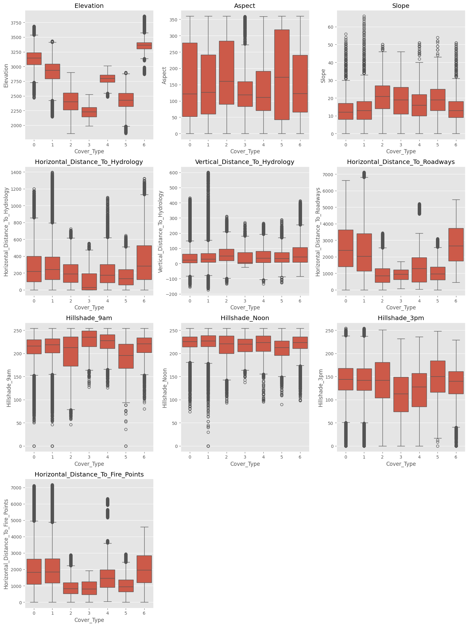
We start as usual with some exploratory data analysis. Most columns contain zeros and ones only; we start from the ones that don’t and plot them, of which we have ten.
numeric_cols = df.select_dtypes(include=[np.number]).columns

numeric_cols = [col for col in numeric_cols if not df[col].isin([0, 1]).all() and col != 'Cover_Type']
n_cols = len(numeric_cols)

assert n_cols > 0, "No numeric columns to visualize"

n_rows = (n_cols + 2) // 3
fig, axes = plt.subplots(n_rows, 3, figsize=(15, 5 * n_rows))
axes = axes.flatten() if n_rows > 1 else [axes]

target = 'Cover_Type'
for i, col in enumerate(numeric_cols):
    sns.boxplot(data=df, x=target, y=col, ax=axes[i])
    axes[i].set_title(f'{col}')

for i in range(n_cols, len(axes)):
    axes[i].set_visible(False)

plt.tight_layout()
n_rows = (n_cols + 2) // 3
fig, axes = plt.subplots(n_rows, 3, figsize=(15, 5 * n_rows))
axes = axes.flatten() if n_rows > 1 else [axes]
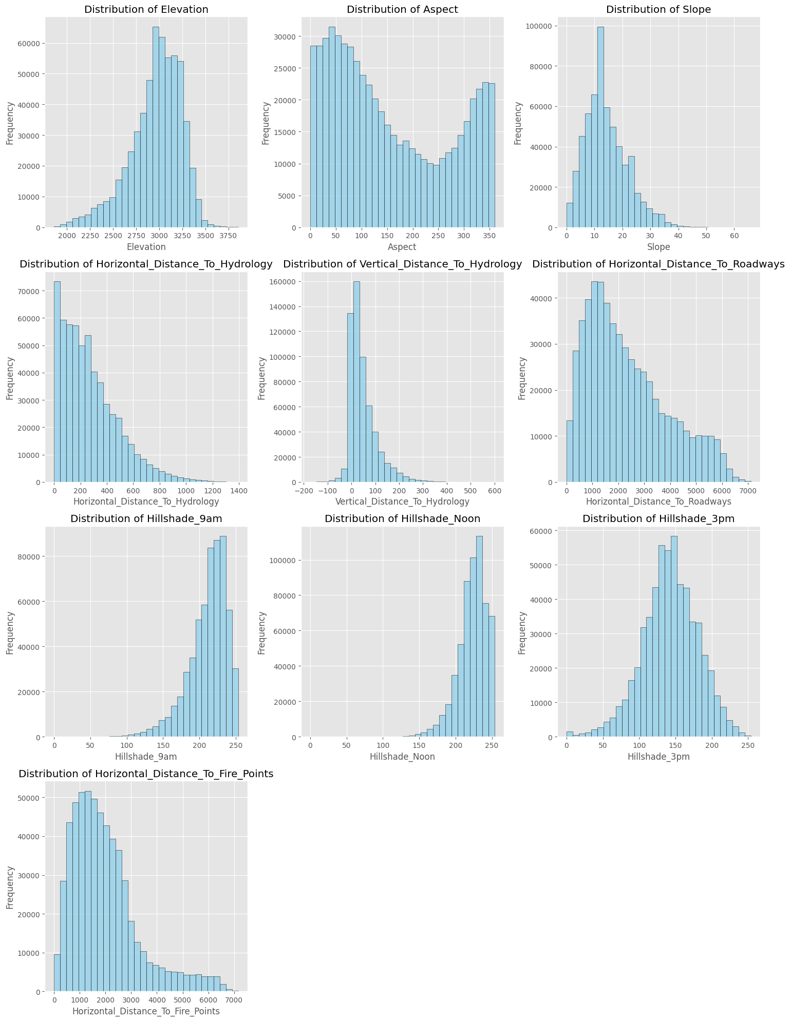
for i, col in enumerate(numeric_cols):
axes[i].hist(df[col], bins=30, alpha=0.7, color='skyblue', edgecolor='black')
axes[i].set_title(f'Distribution of {col}')
axes[i].set_xlabel(col)
axes[i].set_ylabel('Frequency')
for i in range(len(numeric_cols), len(axes)):
axes[i].set_visible(False)
plt.tight_layout()
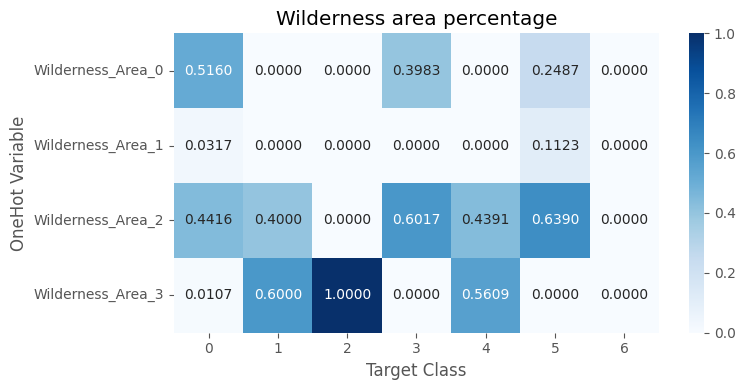
The wilderness area columns are one-hot encoding.
columns = ['Wilderness_Area_0', 'Wilderness_Area_1', 'Wilderness_Area_2', 'Wilderness_Area_3']
# make sure they are a one-hot encoding
assert sum(df[columns].sum(axis='columns') != 1) == 0

result_data = []
for col in columns:
    percentages = (
        df.groupby(target)[col]
            .mean()
            .reindex(range(1, 8), fill_value=0)
            .values
    )
    result_data.append(percentages)

result_df = pd.DataFrame(
    result_data,
    index=columns,
    columns=[str(i) for i in range(0, 7)]
)

plt.figure(figsize=(8, len(columns) * 0.5 + 2))
sns.heatmap(result_df, annot=True, fmt='.4f', cmap='Blues')
plt.xlabel('Target Class')
plt.ylabel('OneHot Variable')
plt.title('Wilderness area percentage')
plt.tight_layout()
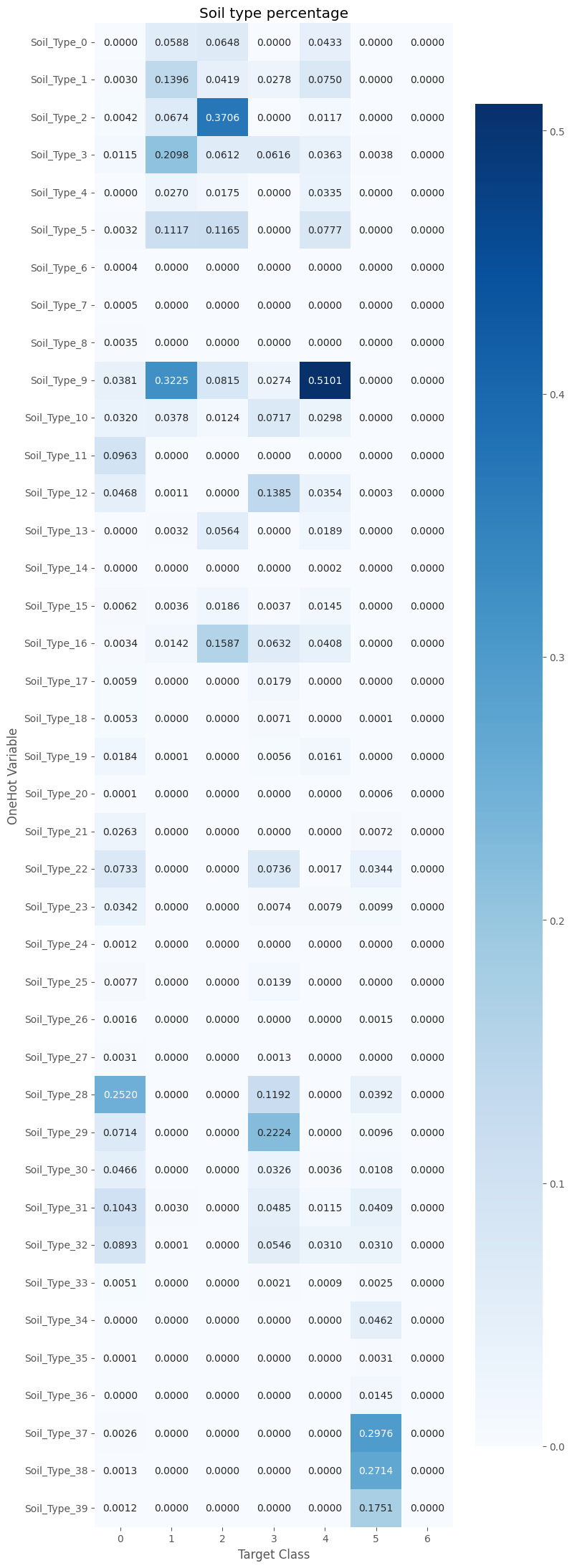
Same is true of the soil type, which is divided into 40 subtypes.
columns = [f'Soil_Type_{i}' for i in range(40)]
# make sure they are a one-hot encoding
assert sum(df[columns].sum(axis='columns') != 1) == 0

result_data = []
for col in columns:
    percentages = (
        df.groupby(target)[col]
            .mean()
            .reindex(range(1, 8), fill_value=0)
            .values
    )
    result_data.append(percentages)

result_df = pd.DataFrame(
    result_data,
    index=columns,
    columns=[str(i) for i in range(0, 7)]
)

plt.figure(figsize=(8, len(columns) * 0.5 + 2))
sns.heatmap(result_df, annot=True, fmt='.4f', cmap='Blues')
plt.xlabel('Target Class')
plt.ylabel('OneHot Variable')
plt.title('Soil type percentage')
plt.tight_layout()
The problem is heavily unbalanced, with almost half of the entries on class #1. This means that a model that always predicts #1 will achieve 48.76% accuracy, and by predicting the first two classes an 87.22% accuracy.
for k, v in df.Cover_Type.value_counts().sort_index().items():
    print(f"Class {k}: {v:>8,} entries ({v / len(df):.2%})")
Class 0:  211,840 entries (36.46%)
Class 1:  283,301 entries (48.76%)
Class 2:   35,754 entries (6.15%)
Class 3:    2,747 entries (0.47%)
Class 4:    9,493 entries (1.63%)
Class 5:   17,367 entries (2.99%)
Class 6:   20,510 entries (3.53%)
from sklearn.model_selection import train_test_split

X = data.data.astype(np.float32)
y = (data.target - 1).astype(np.int64)

# train/test split
X_train, X_test, y_train, y_test = train_test_split(
    X, y, test_size=0.2, random_state=42
)
from sklearn.preprocessing import StandardScaler

scaler = StandardScaler()
X_train = scaler.fit_transform(X_train).astype(np.float32)
X_test  = scaler.transform(X_test).astype(np.float32)
import torch
import torch.nn as nn
import torch.optim as optim
from torch.optim.swa_utils import AveragedModel, SWALR
from torch.utils.data import TensorDataset, DataLoader
from sklearn.metrics import balanced_accuracy_score

train_ds = TensorDataset(torch.tensor(X_train), torch.tensor(y_train))
test_ds  = TensorDataset(torch.tensor(X_test), torch.tensor(y_test))

train_loader = DataLoader(train_ds, batch_size=1_024, shuffle=True)
test_loader  = DataLoader(test_ds, batch_size=1_024)
def get_device():
    if torch.cuda.is_available():
        return 'cuda'
    if torch.mps.is_available():
        return 'mps'
    return 'cpu'
Since the goal of this article is to gather experience with stochastic weight averaging, we use as baseline a simple and small neural network model. A slightly more sophisticated model would improve performances but we’ll stick to the one below.
class MLP(nn.Module):

    def __init__(self):
        super().__init__()
        self.model = nn.Sequential(
            nn.Linear(54, 256),
            nn.ReLU(),
            # nn.BatchNorm1d(256),
            nn.Linear(256, 128),
            nn.ReLU(),
            # nn.BatchNorm1d(512),
            nn.Linear(128, 64),
            nn.ReLU(),
            # nn.BatchNorm1d(64),
            nn.Linear(64, 7)
        )
    def forward(self, x):
        return self.model(x)

device = get_device()
model = MLP().to(device)
criterion = nn.CrossEntropyLoss()

optimizer = optim.SGD(
    model.parameters(), lr=0.1, momentum=0.9, weight_decay=5e-4
)

epochs = 60
swa_start = 30

scheduler = torch.optim.lr_scheduler.CosineAnnealingLR(optimizer, T_max=swa_start)

swa_model = AveragedModel(model).to(device)
swa_scheduler = SWALR(optimizer, swa_lr=0.05)

def evaluate(model, loader, device="cuda"):
    model.eval()
    all_preds = []
    all_labels = []

    with torch.no_grad():
        for Xb, yb in loader:
            Xb, yb = Xb.to(device), yb.to(device)
            preds = model(Xb).argmax(1)

            all_preds.append(preds.cpu().numpy())
            all_labels.append(yb.cpu().numpy())

    all_preds = np.concatenate(all_preds)
    all_labels = np.concatenate(all_labels)

    overall_acc = (all_preds == all_labels).mean()
    balanced_acc = balanced_accuracy_score(all_labels, all_preds)

    # Per-class accuracy (optional)
    class_acc = {}
    for cls in np.unique(all_labels):
        mask = (all_labels == cls)
        class_acc[int(cls)] = (all_preds[mask] == all_labels[mask]).mean()

    return overall_acc, balanced_acc, list(map(float, class_acc.values()))

lrs, sgd_accs, class_accs = [], [], []

from tqdm import trange
for epoch in (p := trange(epochs)):
    model.train()
    for Xb, yb in train_loader:
        Xb, yb = Xb.to(device), yb.to(device)
        optimizer.zero_grad()
        loss = criterion(model(Xb), yb)
        loss.backward()
        optimizer.step()

    # update scheduler
    if epoch > swa_start:
        scheduler.step()
        lrs.append(scheduler.get_last_lr())
    else:
        swa_model.update_parameters(model)
        swa_scheduler.step()
        lrs.append(swa_scheduler.get_last_lr())

    overall_acc, balanced_acc, class_acc = evaluate(model, test_loader, device)
    sgd_accs.append(balanced_acc)
    class_accs.append(class_acc)
    class_acc = ','.join(map(lambda x: f'{x:.2%}', class_acc))
    p.set_description(f"Epoch {epoch+1}/{epochs}: {overall_acc:.4f}/{balanced_acc:.4f}/{class_acc}")

torch.optim.swa_utils.update_bn(train_loader, swa_model, device=device)
swa_overall_acc, swa_balanced_acc, swa_class_acc = evaluate(swa_model, test_loader, device)

print(f"SWA accuracy: {swa_overall_acc:.4f}/{swa_balanced_acc:.4f}/{','.join(map(lambda x: f'{x:.2%}', swa_class_acc))}")
Epoch 60/60: 0.9437/0.8788/93.70%,96.23%,93.92%,74.71%,75.09%,87.47%,94.02%: 100%|██████████| 60/60 [02:30<00:00,  2.51s/it]


SWA accuracy: 0.9329/0.8634/92.26%,95.66%,92.28%,74.52%,71.53%,85.64%,92.50%
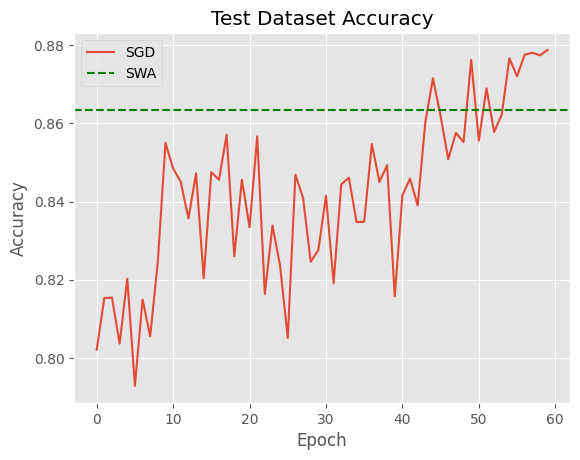
plt.plot(sgd_accs, label='SGD')
plt.xlabel('Epoch')
plt.ylabel('Accuracy')
plt.title("Test Dataset Accuracy")
plt.axhline(y=swa_balanced_acc, linestyle='dashed', color='green', label='SWA')
plt.legend();
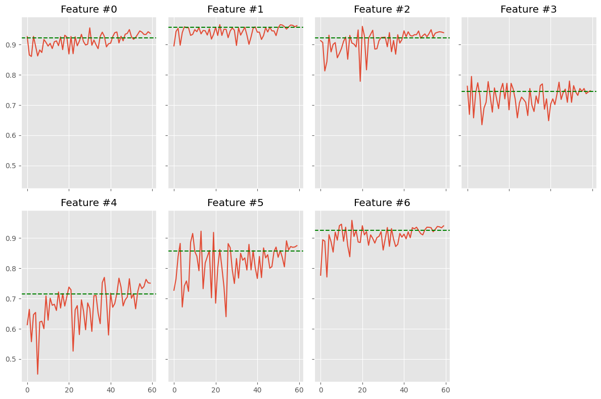
class_accs = np.array(class_accs)
fig, axes = plt.subplots(figsize=(12, 8), nrows=2, ncols=4, sharex=True, sharey=True)
for i, ax in enumerate(axes.ravel()):
    if i < 7:
        ax.plot(class_accs[:, i])
        ax.axhline(y=swa_class_acc[i], color='green', linestyle='dashed')
        ax.set_title(f'Feature #{i}')
    else:
        ax.axis('off')
fig.tight_layout()
In general terms results are not very satisfactory – more sophisticated base models will achieve much higher accuracies. Also, SWA is a bit below the best iterations, so don’t expect to easily improve your model’s performances by using it. The idea, though, is that SWA is more robust and we don’t need to stop convergence at a specific point.