In this post we look at diffusion models, a quite successful class of generative models. A generative model is a model that, given samples from an unknown distribution $p^\star$, is capable of learning a good approximation of it. Once learned, the approximated distribution can be used to generate new samples, or to evaluate the likelihood of observed or sampled data.
In general $p^\star$ is too hard to find directly, so we seek a good approximation of it by defining a sufficiently large parametric family ${ p_\vartheta }_{\vartheta \in \Theta}$, then solve for
\[\vartheta^\star = \argmin_{\vartheta \in \Theta} \mathcal{L}(p_\vartheta, p^\star)\]for some loss function $\mathcal{L}$.
We define $p_\vartheta$ not by using an explicit parametrized distribution family, as they are all too simple for our task, but we rather consider implicitly parametrized probability distributions. That is, we assume some latent variables $z$ and write
\[\begin{aligned} p_\vartheta(x) & = \int p_\vartheta(x, z) dz \\ & = \int p_\vartheta(x \vert z) p_\vartheta(z) dz. \end{aligned}\]The distribution over the latent variables $p_\vartheta(z)$ is generally “simple”, normal or uniform; the complexity of the transformation is contained in $p_\vartheta(x \vert z)$, which is generally based on some deep neural networks functions depending on $z$ for the definition of its coefficients.
With this approach it is easy to sample from $p_\vartheta$:
- first we sample $z \sim p_\vartheta(z)$, which we can do using classical methods for normal or uniform distributions;
- then we compute the coefficients of $p(x \vert z)$ as a function of $z$ and finally we sample $x \sim p_\vartheta(x \vert z)$.
As such, we have defined a generative model.
We still need to define a procedure for computing the optimal parameters $\vartheta^\star$. The approach we follow is to maximize the log-likelihood of our data,
\[\vartheta^\star = \argmax_{\vartheta \in \Theta} \log p_\vartheta(x),\]where $\log p_\vartheta(x)$ is called the evidence. Intuitively, if we have chosen the right $p_\vartheta$ and $\vartheta^\star$, we would expect a high probability of “seeing” our data, and therefore the likelihood will be a “large” number. The classical trick is to define another distribution $q(z)$, and proceed as follows:
\[\begin{aligned} \log p_\vartheta(x) & = \log \int p_\vartheta(x | z) p_\vartheta(z) dz \\ % & = \log \int p_\vartheta(x | z) p_\vartheta(z) \frac{q(z)}{q(z)} dz \\ % & \ge \int \log \left[ p_\vartheta(x | z) \frac{p_\vartheta(z)}{q(z)} \right] q(z) dz \\ % & = \mathbb{E}_q\left[ \log p_\vartheta(x | z) \right] + \mathbb{E}_q\left[ \log \frac{p_\vartheta(z)}{q(z)} \right] \\ % & = \mathbb{E}_q\left[ \log p_\vartheta(x | z) \right] - D_{KL}(q(z) || p_\vartheta(z)). \end{aligned}\]This is called the evidence lower bound, or ELBO. The first term describes the probability of the data $x$ given the latent variables $z$, a quantity we want to maximize by picking those models $q(z)$ that better predict the data. The second term is the negative Kullback-Leibler divergence between $q(z)$ and $p_\vartheta(z)$, and we want to minimize this quantity by choosing $q(z)$ and $p_\vartheta(z)$ to be similar.
The ELBO is quite general and well-known; what changes for diffusion models is the choice of the distributions and the several tricks that make them performant and efficient.
Diffusion models were first presented in Sohl-Dickstein et al., 2015. The key idea of the paper is to use a Markov chain to gradually convert one distribution into another, with each step in the chain analytically tractable – as such, the full chain can also be evaluated. That is, instead of looking for a single transformation that can be difficult to learn and evaluate, we use a composition of several small perturbations. The approach is extended in Ho et al, 2020, which we follow closely for the notation, and further extended in Song et al., 2021.
The basic idea is to start from a given sample, $x_0 \sim p^\star(x_0)$, and using a forward process we define $x_1, x_2, \ldots, x_T$ for some $T > 0$. With a small abuse of notation, $x_0$ is our actual data while $x_1, \ldots, x_T$ are latent variables into which the data in transformed. (That is, we use $x$ for both the data and the latent variables.) At each step $t$ a bit or noise is added, until when, at $t=T$, the data becomes indistinguishable from pure Gaussian noise. A second process, the reverse process, will then generate data starting from pure Gaussian noise, thus going from $t=T$ to $t=0$.
More formally and using $x \sim \mathcal{N}(x; \mu, \sigma^2 I)$ to indicate a multivariate sample $x$ of a normal distribution with mean $\mu$ and diagional variance matrix $\sigma^2$, we define the forward diffusion process that adds a small amount of Gaussian noise to the sample in $T$ steps producing a sequence of noisy samples $x_1, \ldots, x_T$ as follows. Given a variance schedule ${ \beta_t \in (0, 1) }_{t=1}^T$, we have
\[q(x_t | x_{t-1}) = \mathcal{N} \left(x_t; \sqrt{1 - \beta_t} x_{t-1}, \beta_t I \right)\]and
\[q(x_1, \cdots, x_T | x_0) = \Pi_{t=1}^T q(x_t | x_{t-1}).\]The values of $T$ and $\beta_t$ must be defined such that the distribution of $x_T$ is close to normal. In general the variance schedule $\beta_t$ is not learnt and given.
If we could sample from $q(x_{t - 1} \vert x_t)$, we could reverse the process and generate samples from Gaussian noise. Unfortunately we cannot easily estimate it directly but we can set up a model that learns such transformation. We define such reverse process as
\[p_\vartheta(x_0, \ldots, x_T) = p(x_T) \Pi_{t=1}^T p_\vartheta(x_{t-1} \vert x_t)\]with
\[p_\vartheta(x_{t-1} | x_t) = \mathcal{N}\left(x_{t-1} | \mu_\vartheta(x_t, t), \Sigma_\vartheta(x_t, t)\right)\]and
\[p_x(_T) = \mathcal{N}(x_T; 0, I).\]Graphically, the behavior is as below, with the $q$ distributions moving forward from $x_0$ to $x_T$ and the $p_\vartheta$ distributions moving backward from $x_T$ to $x_0$:
\[x_0 \xrightleftarrows[\displaystyle p_\vartheta(x_0 | x_1)]{\displaystyle q(x_1 | x_0)} x_1 \quad \cdots \quad x_{t-1} \xrightleftarrows[\displaystyle p_\vartheta(x_{t-1} | x_t)]{\displaystyle q(x_t | x_{t-1})} x_t \quad \cdots \quad x_{T-1} \xrightleftarrows[\displaystyle p_\vartheta(x_{T-1} | x_T)]{\displaystyle q(x_T | x_{T-1})} x_T.\]To define the loss function for a given point $x_0$ we use the ELBO to define the loss function for the minimization problem:
\[\begin{aligned} -\log p_\vartheta(x_0) & = - \log \int p_\vartheta(x_0, x_1, x_2, \ldots, x_T) dx_1 dx_2 \cdots dx_T \\ % & = - \log \int \frac{p_\vartheta(x_0, x_1, \ldots, x_T) q(x_1, \ldots, x_T | x_0)}{q(x_1, \cdots, x_T | x_0)} dx_{1:T} \\ % & = -\log \mathbb{E}_{q(x_1, \ldots, x_T)} \left[ \frac{p_\vartheta(x_0, x_1, \ldots, x_T)}{q(x_1, \ldots, x_T) | x_0)} \right] \\ % & \le -\mathbb{E}_{q(x_1, \ldots, x_T)}\left[ \log \frac{p_\vartheta(x_0, x_1, \ldots, x_T)}{q(x_1, \ldots, x_T | x_0)} \right] \\ % & = -\mathbb{E}_{q(x_1, \ldots, x_T)}\left[ \log \frac{ p(x_T) \Pi_{t=1}^T p_\vartheta(x_{t-1} | x_t) }{ \Pi_{t=1}^T q(x_t | x_{t-1}) } \right] \\ % & = - \mathbb{E}_{q(x_T)}[p(x_T)] + \sum_{t=1}^T D_{KL} \left(q(x_t | x_{t-1} \,||\, p_\vartheta(x_{t-1} | x_t)) \right). \end{aligned}\]Since there are no learnable parameters in $p(x_T)$, our loss function will be
\[\mathcal{L} = \sum_{t=1}^T D_{KL} \left(q(x_t | x_{t-1}) \,||\, p_\vartheta(x_{t-1} | x_t)\right).\]Once the forward process is known, the KL-divergence above is easy to compute because both $q(x_t | x_{t-1})$ and $p_\vartheta(x_{t-1} | x_t)$ are normal. That is, since $x_{t-1}$ is known, we can compute the mean and variance of the normal distribution that defines $q$; the same holds for $p_\vartheta$ given that $x_t$ is known as well.
This is the most basic formulation of the method, which we will use in the code below.
import matplotlib.pyplot as plt
import matplotlib as mpl
import pandas as pd
import numpy as np
import torch
import itertools
from tqdm.auto import tqdm
np.random.seed(42)
_ = torch.manual_seed(43)
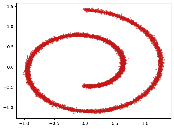
We use the two-dimensional version of the swiss roll dataset. This is often use as a test in nonlinear dimensionality reduction; here we are interested in the distribution of its points, which we want to be able to reproduce using diffusion methods. Each entry $x$ in our dataset is composed by two values, the X-axis component and the Y-axis component. We use 10’000 such points; the scatter plot explains the name of the dataset. The coordinates are scaled by a factor 10 to be more unitary in magnitude.
from sklearn.datasets import make_swiss_roll
num_samples = 10_000
dataset, _ = make_swiss_roll(num_samples, noise=0.2)
dataset = dataset[:, (0, 2)] / 10
plt.scatter(dataset[:, 0], dataset[:, 1], alpha=0.5, color='red', edgecolor='firebrick', s=5)
dataset = torch.Tensor(dataset).float()
We use $T=50$ and a constant $\beta_t=0.05^2$.
T = 50
β_all = 0.05**2 * np.ones(T)
The forward process is used to move from the input $x_0 = x$ to the noisy version $x_T$. We store the distributions as well as the realizations to compute the log probabilities in the loss function.
def compute_forward_process(x_0, T=T, β_all=β_all):
    q_all, x_all = [None], [x_0]
    x_t = x_0
    for t in range(T):
        β_t = β_all[t]
        q_t = torch.distributions.Normal(np.sqrt(1 - β_t) * x_t, np.sqrt(β_t))
        x_t = q_t.sample()
        q_all.append(q_t)
        x_all.append(x_t)
    return q_all, x_all
The function plot_evolution() allows us to see ten steps of the transformation from $x_0$ to $x_T$. We can see that our swiss roll becomes more or more Gaussian.
def plot_evolution(x_all, is_reverse=False):
    fig, axes = plt.subplots(1, 11, figsize=(33, 3), sharex=True, sharey=True)
    for i in range(11):
        t = i * 5
        x_t = x_all[t]
        axes[i].scatter(x_t[:, 0], x_t[:, 1], color='grey', edgecolor='blue', s=5);
        axes[i].set_xticks([-1, 1])
        axes[i].set_yticks([-1, 1])
        label = T - t if is_reverse else t
        if label == T: label = 'T'
        axes[i].set_title(f't={label}')
        axes[i].axis('square')
    fig.tight_layout()
_, x_all = compute_forward_process(dataset[:1_000])
plot_evolution(x_all)

The reverse process requires the definition of two models, one for $\mu_\vartheta(x_t, t)$ and the other for $\Sigma_\vartheta(x_t, t)$ for the standard deviation. The input size is three – the two spatial dimensions plus time, while the output has two dimensions. We keep the same structure for both mean and standard deviation, with the only addition of a softplus function to the standard deviation one.
μ_model = torch.nn.Sequential(
    torch.nn.Linear(2 + 1, 128),
    torch.nn.ReLU(),
    torch.nn.Linear(128, 128),
    torch.nn.ReLU(),
    torch.nn.Linear(128, 128),
    torch.nn.ReLU(),
    torch.nn.Linear(128, 2)
)

σ_model = torch.nn.Sequential(
    torch.nn.Linear(2 + 1, 128),
    torch.nn.ReLU(),
    torch.nn.Linear(128, 128),
    torch.nn.ReLU(),
    torch.nn.Linear(128, 128),
    torch.nn.ReLU(),
    torch.nn.Linear(128, 2),
    torch.nn.Softplus()
)
The computation of the reverse process is similar to the one of the forward process, but it uses the two models for mean and standard deviation at each step.
def compute_reverse_process(μ_model, σ_model, count, T=T):
    p = torch.distributions.Normal(torch.zeros(count, 2), torch.ones(count, 2))
    x_t = p.sample()
    sample_history = [x_t]
    for t in range(T, 0, -1):
        xin = torch.cat((x_t, (t / T) * torch.ones(x_t.shape[0], 1)), dim=1)
        p = torch.distributions.Normal(μ_model(xin), σ_model(xin))
        x_t = p.sample()
        sample_history.append(x_t)
    return sample_history
As customary, we define a tiny class that wraps our dataset.
class MyDataset(torch.utils.data.Dataset):

    def __init__(self, X):
        super().__init__()
        self.X = X

    def __len__(self):
        return self.X.shape[0]

    def __getitem__(self, index):
        return self.X[index]
It is a good practice to initialize the weights of the model – here we use Xavier initialization
def init_weights(m):
    if isinstance(m, torch.nn.Linear):
        torch.nn.init.xavier_uniform_(m.weight)
        m.bias.data.fill_(0.01)

for model in [μ_model, σ_model]:
    model.apply(init_weights)
The compute_loss() function contains all the logic of the method. This implementation is not very efficient but it reflects the formulae we have seen above and it is a nice starting point to understand those methods. The inputs are all the steps of the forward process as well as all the corresponding distributions, plus the models for $\mu_\vartheta$ and $\Sigma_\vartheta$. Using those inputs we can easily compute the various terms we need: $\log p(x_T)$, $\log p_\vartheta(x_{t-1} \vert x_t)$ and $\log q(x_{t} \vert x_{t-1})$. The integrals are approximated by the average over all the samples.
def compute_loss(q_all, x_all, μ_model, σ_model):
    p = torch.distributions.Normal(
        torch.zeros(x_all[0].shape),
        torch.ones(x_all[0].shape)
    )

    loss = -p.log_prob(x_all[-1]).mean()

    for t in range(1, T):
        x_t = x_all[t]
        x_t_minus_1 = x_all[t - 1]
        q_t = q_all[t]

        x_input = torch.cat((x_t, (t / T) * torch.ones(x_t.shape[0], 1)), dim=1)
        p_t_minus_1 = torch.distributions.Normal(μ_model(x_input), σ_model(x_input))

        loss -= torch.mean(p_t_minus_1.log_prob(x_t_minus_1))
        loss += torch.mean(q_t.log_prob(x_t))

    return loss / T
params = itertools.chain(μ_model.parameters(), σ_model.parameters())
optim = torch.optim.Adam(params, lr=1e-3)
data_loader = trainloader = torch.utils.data.DataLoader(MyDataset(dataset), batch_size=512, shuffle=True)

loss_history = []
bar = tqdm(range(1, 1000 + 1))
for e in bar:

    for x_0 in data_loader:
        forward_distributions, forward_samples = compute_forward_process(x_0)

        optim.zero_grad()
        loss = compute_loss(forward_distributions, forward_samples, μ_model, σ_model)
        loss.backward()
        torch.nn.utils.clip_grad_norm_(params, 1)
        optim.step()
        bar.set_description(f'Loss: {loss.item():.4f}')
        loss_history.append(loss.item())

    if e in [1, 10, 20, 50] or e % 100 == 0:
        with torch.no_grad():
            print(f'iter: {e}, loss: {loss.item():.6e}')
            x_all = torch.stack(compute_reverse_process(μ_model, σ_model, 200))
            plot_evolution(x_all, True)
            plt.show()
  0%|          | 0/1000 [00:00<?, ?it/s]


iter: 1, loss: 8.050011e-01

iter: 10, loss: 2.388238e-02

iter: 20, loss: 2.569752e-02

iter: 50, loss: 2.346585e-02

iter: 100, loss: 1.600004e-02

iter: 200, loss: 1.569699e-02

iter: 300, loss: 1.637200e-02

iter: 400, loss: 5.513587e-03

iter: 500, loss: 7.712739e-03

iter: 600, loss: 8.991304e-03

iter: 700, loss: 5.626636e-03

iter: 800, loss: 9.135569e-03

iter: 900, loss: 4.601617e-03

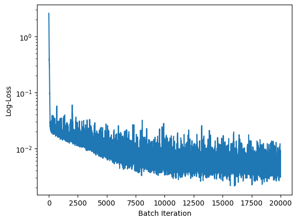
iter: 1000, loss: 3.721235e-03

plt.semilogy(loss_history)
plt.xlabel('Batch Iteration')
plt.ylabel('Log-Loss');
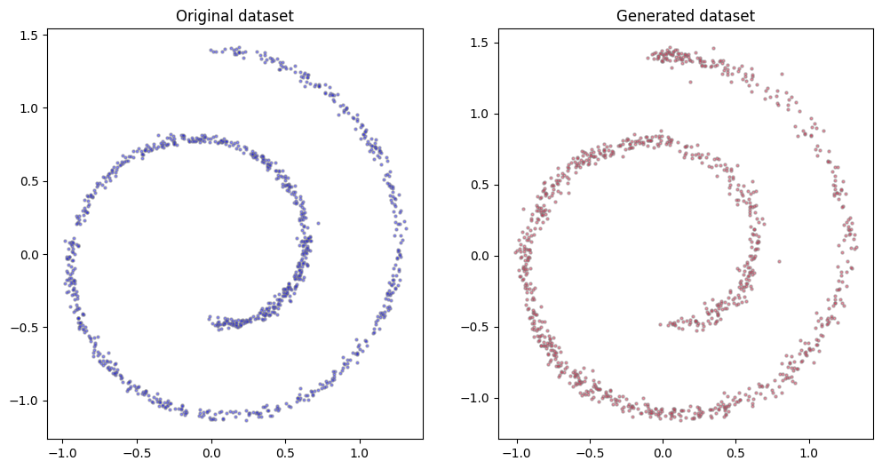
Results aren’t bad, even if they are not too good neither, with the generated dataset being a bit more diffused than the original one. In my tests different learning rates, number of steps $T$ or number of points in the neural networks didn’t change the results substantially.
fig, (ax0, ax1) = plt.subplots(figsize=(12, 6), ncols=2)
n = 1_000
ax0.scatter(dataset[:n, 0], dataset[:n, 1], alpha=0.5, color='blue', edgecolor='grey', s=5)
ax0.set_title('Original dataset')
x_all = torch.stack(compute_reverse_process(μ_model, σ_model, n))
ax1.scatter(x_all[-1][:, 0], x_all[-1][:, 1], alpha=0.5, color='crimson', edgecolor='grey', s=5)
ax1.set_title('Generated dataset');
To improve the results we can leverage on the properties of the forward process. First note that, being the composition of normal transformations, the forward process admits sampling $x_t$ at an arbitrary time $t$ in closed form. In fact, using the notation $\alpha_t = 1- \beta_t$ and $\varepsilon_i \sim \mathcal{N}(0, 1)$, we have
\[\begin{aligned} x_1 & = \sqrt{\alpha_0} \, x_0 + \sqrt{1 - \alpha_0} \, \varepsilon_1 \\ % x_2 & = \sqrt{\alpha_1} \, x_1 + \sqrt{1 - \alpha_0} \, \varepsilon_2 \\ % & = \sqrt{\alpha_0} \sqrt{\alpha_1} \, x_0 + \sqrt{\alpha_2} \sqrt{1 - \alpha_1} \varepsilon_1 + \sqrt{1 - \alpha_2} \, \varepsilon_2 \\ % & = \sqrt{\alpha_0 \alpha_1} \, x_0 + \sqrt{\alpha_2(1 - \alpha_1) + 1 - \alpha_2} \, \varepsilon_{1,2} \\ % & = \sqrt{\alpha_0 \alpha_1} \, x_0 + \sqrt{1 - \alpha_1 \alpha_2} \, \varepsilon_{1,2} \\ % x_3 & = \sqrt{\alpha_3} \, x_2 + \sqrt{1 - \alpha_3} \, \varepsilon_3 \\ % & = \sqrt{\alpha_1 \alpha_2 \alpha_3} \, x_0 + \sqrt{1 - \alpha_1 \alpha_2 \alpha_3} \, \varepsilon_3 \\ % x_t & = \sqrt{\bar{\alpha}_t} \, x_0 + \sqrt{1 - \bar \alpha_t} \, \varepsilon_t, \end{aligned}\]that is,
\[x_t \sim \mathcal{N} \left( x_t; \sqrt{\bar{\alpha}_t} \, x_0, (1 - \bar\alpha_t) I \right),\]where $\bar\alpha_t = \Pi_{s=1}^t \alpha_s = \Pi_{s=1}^t (1 - \beta_s)$.
The second important observation is that, due to the Markov property,
\[q(x_t | x_{t-1}) = q(x_t | x_{t-1}, x_0)\]because $0 \le t - 1$. Using Bayes’ rule, we have
\[q(x_{t-1} | x_t, x_0) = \frac{q(x_t | x_{t - 1}, x_0) q(x_{t - 1} | x_0)}{q(x_t | x_0)}.\]This means that we have two ways of expressing the reverse process, one using $p_\vartheta$ and the other using $q$. The latter only works when conditioned on $x_0$, henceforth it is not useful to generate a new $x_0$ – we would need to know $x_0$ to generate it. However this suggests a new approach: if we can find an expression for $q(x_{t-1} \vert x_t, x_0)$, we could train $p_\vartheta$ to learn it for several $x_0$, then use it to generate new $x_0$.
\[x_0 \xrightleftarrows[ {\displaystyle p_\vartheta(x_0 \vert x_1)} \atop {\displaystyle q(x_0 \vert x_1, x_0)} ]{\displaystyle q(x_1 \vert x_0)} x_1 \quad \cdots \quad x_{t-1} \xrightleftarrows[ {\displaystyle p_\vartheta(x_{t-1} \vert x_t)} \atop {\displaystyle q(x_{t-1} \vert x_t, x_0)} ]{\displaystyle q(x_t \vert x_{t-1})} x_t \quad \cdots \quad x_{T-1} \xrightleftarrows[ {\displaystyle p_\vartheta(x_{T-1} \vert x_T)} \atop {\displaystyle q(x_{T-1} \vert x_T, x_0)} ]{\displaystyle q(x_T \vert x_{T-1})} x_T.\]We already know the expression for $q(x_t \vert x_{t-1}, x_0) = q(x_t \vert x_{t-1})$. Thanks to the property of the previous paragraph we have
\[q(x_t | x_0) = \mathcal{N}(x_t; \sqrt{\bar{\alpha}_t} x_0, (1 - \bar{\alpha}_t)I).\]All the three expressions on the right-hand side of Bayes’ rule are normal distributions,
\[\begin{aligned} q(x_{t-1} | x_t, x_0) & = \frac{ \mathcal{N}\left( x_t; \sqrt{\alpha_t} x_{t-1}, (1 - \alpha_t) I \right) \mathcal{N}\left( x_{t-1}; \sqrt{\bar\alpha_{t-1}} x_0, (1 - \bar\alpha_{t-1} ) I\right) }{ \mathcal{N}\left( x_t; \sqrt{\bar\alpha_t} x_0, (1 - \bar\alpha_t ) I\right) } \\ % -- & \propto \exp\left\{ -\left[ \frac{(x_t - \sqrt{\alpha_t} \, x_{t-1})^2}{2(1 - \alpha_t)} + \frac{(x_{t-1} - \sqrt{\bar\alpha_{t-1}}\, x_0)^2}{2(1 - \bar\alpha_{t-1})} - \frac{(x_t - \sqrt{\bar\alpha_t} \, x_0)^2}{2(1 - \bar\alpha_t)} \right] \right\} \\ % -- & = \exp\left\{ -\frac{1}{2} \left[ \frac{(x_t - \sqrt{\alpha_t} \, x_{t-1})^2}{1 - \alpha_t} + \frac{(x_{t-1} - \sqrt{\bar\alpha_{t-1}}\, x_0)^2}{1 - \bar\alpha_{t-1}} - \frac{(x_t - \sqrt{\bar\alpha_t} \, x_0)^2}{1 - \bar\alpha_t} \right] \right\} \\ % -- & = \exp\left\{ -\frac{1}{2} \left[ \frac{-2x_t \sqrt{\alpha_t} \, x_{t-1} + \alpha_t x_{t-1}^2 }{1 - \alpha_t} + \frac{x_{t-1}^2 - 2 x_{t-1}\sqrt{\bar\alpha_{t-1}} x_0}{1 - \bar\alpha_{t-1}} + C(x_t, x_0) \right] \right\} \\ % -- & \propto \exp\left\{ -\frac{1}{2} \left[ - \frac{-2 \sqrt{\alpha_t} \, x_t x_{t-1}}{1 - \alpha_t} + \frac{\alpha_t x_{t-1}^2 }{1 - \alpha_t} + \frac{x_{t-1}^2}{1 - \bar\alpha_{t-1}} % - \frac{2 \sqrt{\bar\alpha_{t-1}} \, x_{t-1} x_0}{1 - \bar\alpha_{t-1}} \right] \right\} \\ % -- & = \exp\left\{ -\frac{1}{2} \left[ \frac{\alpha_t(1-\bar\alpha_{t-1}) + 1 - \alpha_t}{(1 - \alpha_t) (1 - \bar\alpha_{t-1})} x_{t-1}^2 - 2 \left( \frac{\sqrt{\alpha_t} x_t}{1 - \alpha_t} + \frac{\sqrt{\bar\alpha_{t-1}} \, x_0}{1 - \bar\alpha_{t-1}} \right) x_{t-1} \right] \right\} \\ % -- & = \exp\left\{ -\frac{1}{2} \left[ \frac{1 - \bar\alpha_t}{(1 - \alpha_t) (1 - \bar\alpha_{t-1})} x_{t-1}^2 - 2 \left( \frac{\sqrt{\alpha_t} x_t}{1 - \alpha_t} + \frac{\sqrt{\bar\alpha_{t-1}} \, x_0}{1 - \bar\alpha_{t-1}} \right) x_{t-1} \right] \right\} \\ % -- & = \exp\left\{ -\frac{1}{2} \frac{1 - \bar\alpha_t}{(1 - \alpha_t) (1 - \bar\alpha_{t-1})} \left[ x_{t-1}^2 - 2 \frac{ \frac{\sqrt{\alpha_t}}{1 - \alpha_t} x_t + \frac{\sqrt{\bar\alpha_{t-1}}}{1-\bar\alpha_{t-1}} x_0 }{ \frac{1 - \bar\alpha_t}{(1 - \alpha_t) (1 - \bar\alpha_{t-1})} } x_{t-1} \right] \right\} \\ % -- & = \exp\left\{ - \frac{1}{2 \Sigma^2_q(t)} \left[ x_{t-1}^2 - 2 \frac{ \sqrt{\alpha_t} (1 - \bar\alpha_{t-1}) \, x_t + \sqrt{\bar\alpha_{t-1}} (1 - \alpha_t) x_0 }{ 1 - \bar\alpha_t } x_{t-1} \right] \right\} \\ % -- & \propto \mathcal{N} \left( x_{t-1}; \mu_q(x_t, x_0), \Sigma_q^2 (x_t, x_0) \right). \end{aligned}\]This means that we can express $q(x_{t-1} \vert x_t, x_0)$ with a normal distribution with mean $\mu_q(x_t, x_0)$ and variance $\Sigma_q^2(t)$ given by the expressions
\[\begin{aligned} \mu_q(x_t, x_0) & = \frac{ \sqrt{\alpha_t} (1 - \bar\alpha_{t-1}) \, x_t + \sqrt{\bar\alpha_{t-1}} (1 - \alpha_t) x_0 }{ 1 - \bar\alpha_t } \\ % \Sigma_q^2(t) & = \frac{(1 - \alpha_t) (1 - \bar\alpha_{t-1})}{1 - \bar\alpha_t}. \end{aligned}\]In order to match the approximate denoising transitions $p_\vartheta(x_{t-1} \vert x_t)$ to the ground-truth denoising transition step $q(x_{t-1} \vert x_t, x_0)$ as close as possile, it makes sense to model it as a Gaussian distribution, which is what we have done. As suggested in [Ho et al., 2020], we simplify the reverse process by choosing $\Sigma_q(t) = \sigma_t I$. Our loss function will then minimize the Kullback-Leibler distance between the two distributions,
\[\begin{aligned} \mathcal{L}_t & = D_{KL}(q(x_{t-1} \vert x_t, x_0) || p_\vartheta(x_{t-1}, x_t)) \\ % --- & \propto D_{KL}(\mathcal{N}(x_{t-1}; \mu_q(x_t, t), \Sigma^2_q(t) || \mathcal{N}(x_{t-1}; \mu_\vartheta(x_t, t), \Sigma_\vartheta(x_t, t))) \\ % --- & = \frac{1}{2}\left[ \log \frac{\vert\Sigma^2_q(t)\vert}{\vert\Sigma^2_q(t)\vert} - d + \operatorname{tr} \left(\Sigma^2_q(t)^{-1} \Sigma^2_q(t) \right) + \left( \mu_\vartheta(x_t, t) -\mu_q(x_t, t) \right)^T \Sigma^2_q(t)^{-1} (\mu_\vartheta(x_t, t) -\mu_q(x_t, t)) \right] \\ % --- & = \frac{1}{2} \left[ \log 1 - d + d + \Sigma_q^2(t)^{-1} \left( \mu_\vartheta(x_t, t) -\mu_q(x_t, t) \right)^T \left( \mu_\vartheta(x_t, t) -\mu_q(x_t, t) \right) \right] \\ % --- & = \frac{1}{2 \Sigma_q^2(t)} \vert \mu_\vartheta(x_t, t) - \mu_q(x_t, t) \vert^2, \end{aligned}\]that is, we want to find a $\mu_\vartheta(x_t, t)$ that matches $\mu_q(x_t, t)$. Noting that
\[x_t = \sqrt{\bar\alpha_t} \, x_0 + \sqrt{1 - \bar\alpha_t} \, \varepsilon_t\]we can express $x_0$ as
\[x_0 = \frac{1}{\sqrt{\bar\alpha_t}}\left( x_t - \sqrt{1 - \bar\alpha_t} \, \varepsilon_t \right).\]Plugging the above expressions for $x_0$ in the definitions of $\mu_q$, we obtain
\[\begin{aligned} \mu_q(x_t, x_0, t) & = % \frac{\sqrt{\alpha_t}(1 - \bar\alpha_{t-1}) x_t}{1 - \bar\alpha_t} + \frac{\sqrt{\bar\alpha_{t-1}}(1 - \alpha_t)}{1 - \bar\alpha_t} \frac{1}{\sqrt{\alpha_t}} \left( x_t - \sqrt{1 - \bar\alpha_t \, \varepsilon_t} \right) \\ % & = \frac{1}{\sqrt{\alpha_t}} \left( x_t - \frac{1 - \alpha_t}{\sqrt{1 - \bar\alpha_t}} \varepsilon_t \right). \end{aligned}\]We can go back to our loss function,
\[\begin{aligned} \mathcal{L} & = \mathbb{E}_{q(x_1, \ldots, x_T)}\left[ \log \frac{ \Pi_{t=1}^T q(x_t | x_{t-1}) }{ p(x_T) \Pi_{t=1}^T p_\vartheta(x_{t-1} | x_t) } \right] \\ % --- & = \mathbb{E}_{q(x_1, \ldots, x_T)}\left[ -\log p(x_T) + \sum_{t=1}^T \log \frac{ q(x_t | x_{t-1}) }{ p_\vartheta(x_{t-1} | x_t) } \right] \\ % --- & = \mathbb{E}_{q(x_1, \ldots, x_T)}\left[ -\log p(x_T) + \sum_{t=2}^T \log \frac{ q(x_t | x_{t-1}) }{ p_\vartheta(x_{t-1} | x_t) } + \log \frac{q(x_1 | x_0)}{p_\vartheta(x_0 | x_1)} \right] \\ % --- & = \mathbb{E}_{q(x_1, \ldots, x_T)}\left[ -\log p(x_T) + \sum_{t=2}^T \log \frac{ q(x_t | x_{t-1}, x_0) }{ p_\vartheta(x_{t-1} | x_t) } + \log \frac{q(x_1 | x_0)}{p_\vartheta(x_0 | x_1)} \right] \\ % --- & = \mathbb{E}_{q(x_1, \ldots, x_T)}\left[ -\log p(x_T) + \sum_{t=2}^T \log \frac{ q(x_{t-1} | x_t, x_0) }{ p_\vartheta(x_{t-1} | x_t) } \frac{q(x_t | x_0)}{q(x_{t-1} | x_0)} + \log \frac{q(x_1 | x_0)}{p_\vartheta(x_0 | x_1)} \right] \\ % --- & = \mathbb{E}_{q(x_1, \ldots, x_T)}\left[ -\log p(x_T) + \sum_{t=2}^T \log \frac{ q(x_{t-1} | x_t, x_0) }{ p_\vartheta(x_{t-1} | x_t) } + \sum_{t=2}^T \log \frac{q(x_t | x_0)}{q(x_{t-1} | x_0)} + \log \frac{q(x_1 | x_0)}{p_\vartheta(x_0 | x_1)} \right] \\ % --- & = \mathbb{E}_{q(x_1, \ldots, x_T)}\left[ -\log p(x_T) + \sum_{t=2}^T \log \frac{ q(x_{t-1} | x_t, x_0) }{ p_\vartheta(x_{t-1} | x_t) } + \log \frac{q(x_T | x_0)}{q(x_{1} | x_0)} + \log \frac{q(x_1 | x_0)}{p_\vartheta(x_0 | x_1)} \right] \\ % --- & = \mathbb{E}_{q(x_1, \ldots, x_T)}\left[ \underbrace{\log \frac{q(x_T | x_0)}{p(x_T)}}_{\mathcal{L}_T} + \sum_{t=2}^T \underbrace{\log \frac{q(x_{t-1} | x_t, x_0)}{p_\vartheta(x_{t-1} | x_t)}}_{\mathcal{L}_{t-1}} - \underbrace{\log p_\vartheta(x_0 | x_1)}_{\mathcal{L}_0} \right] \\ \end{aligned}\]The first terms does not depend on the parameters $\vartheta$ and can be ignored in the optimization. The second term, with a summation from $i=2$ to $T$, compare two normal distributions and can therefore be computed in closed form,
\[\mathcal{L}_t = \frac{1}{2 \Sigma_q^2(t)} \| \mu_q(x_t, t) - \mu_\vartheta(x_t, t) \|^2.\]As explained in Section 3.2 of Ho et al, 2020, we can simplify this expression further. First, we write
\[x_t(x_0, \varepsilon) = \sqrt{\bar\alpha_t} \, x_0 + \sqrt{1 - \bar\alpha_t} \varepsilon,\]meaning that the difference term in our loss function can be rewritten as
\[\mu_q \left(x_t(x_0, \varepsilon, t), \frac{1}{\sqrt{\bar\alpha_t}} x_0 + \sqrt{1 - \bar\alpha_t} \, \varepsilon \right) - \mu_\vartheta(x_t(x_0, t), t).\]That is, $\mu_\vartheta$ must predict
\[\mu_q \left(x_t(x_0, \varepsilon, t), \frac{1}{\sqrt{\bar\alpha_t}} x_0 + \sqrt{1 - \bar\alpha_t} \, \varepsilon \right)\]given $x_t$. Since $x_t$ is available as input to the model, we choose the parametrizatin
\[\mu_\vartheta(x_t(x_0, t), t) = \frac{1}{\sqrt{\alpha_t}} \left( x_t - \frac{1 - \alpha_t}{\sqrt{1 - \bar\alpha_t}} \varepsilon_\vartheta(x_t, t) \right)\]where $\varepsilon_\vartheta(x_t, t)$ aims to predict $\epsilon$ from $x_t$ and $t$. The loss function simplifies to
\[\mathcal{E}_{x_0, \varepsilon} \left[ \frac{\beta_t^2}{2 \sigma_t^2 \alpha_t (1 - \bar\alpha_t)} \left\| \varepsilon - \varepsilon_\vartheta\left( \sqrt{\bar\alpha_t} x_0 + \sqrt{1 - \bar\alpha_t} \, \varepsilon, t \right) \right\|^2 \right]\]The training algorithm (top of page 4 of Ho et al, 2020) becomes the following:
- Do:
- $\quad\quad x_0 \sim p^\star (x_0)$
- $\quad\quad t \sim \mathcal{U} ({1, \ldots, T})$
- $\quad\quad \varepsilon \sim \mathcal{N}(0, I)$
- $\quad\quad \mathcal{L}\vartheta() = \left\lVert \varepsilon - \varepsilon\vartheta \left( \sqrt{\bar\alpha_t} \, x_0 + \sqrt{1 - \bar\alpha_t}\,\varepsilon, t \right) \right\rVert$
- Compute $\nabla_\vartheta \mathcal{L}_\vartheta$ and perform one optimization step
- If converged then stop
To generate a new sample we compute the reverse process:
- $x_T \sim \mathcal{N}(0, I)$
- For $t=T, \ldots, 1$ do:
- $\quad\quad z \sim \mathcal{N}(0, I) \text{ if } t > 0 \text{ else } z = 0$
- $\quad\quad x_{t-1} = \frac{1}{\sqrt{\alpha_t}}\left( x_t - \frac{1 - \alpha_t}{\sqrt{1 - \bar\alpha_t}} \varepsilon_\vartheta(x_t, t) \right) + \sigma \sqrt{1 - \alpha_t} z$
- End For
- Return $x_0$
We will now code this improved approach. The code is similar yet the convergence much faster, due to the reduced variance. We will use $T=250$ and $\beta_t = 0.025^2$. Some of the utility functions defined above are redefined here.
import torch.nn.functional as F
T = 250
β_all = 0.025**2 * torch.ones(T + 1)
α_all=1 - β_all
ᾱ_all = torch.cumsum(α_all.log(), dim=0).exp()
ᾱ_all[0] = 1
def compute_forward_process(x_0, t):
    ε = torch.randn_like(x_0)
    ᾱ_t = ᾱ_all[t].unsqueeze(-1)
    return ᾱ_t.sqrt() * x_0 + (1 - ᾱ_t).sqrt() * ε, ε
def plot_evolution(x_all, is_reverse=False):
    fig, axes = plt.subplots(1, 11, figsize=(33, 3), sharex=True, sharey=True)
    for i in range(11):
        t = i * 25
        x_t = x_all[t]
        axes[i].scatter(x_t[:, 0], x_t[:, 1], color='grey', edgecolor='blue', s=5);
        axes[i].set_xticks([-1, 1])
        axes[i].set_yticks([-1, 1])
        label = T - t if is_reverse else t
        if label == T: label = 'T'
        axes[i].set_title(f't={label}')
        axes[i].axis('square')
    fig.tight_layout()
tmp = [compute_forward_process(dataset[:1_000], t)[0] if t != -1 else dataset for t in range(-1, T)]
plot_evolution(tmp)

def backward(x, t, pred_noise, z):
    if z is None:
        z = torch.randn_like(x)
    noise = β_all.sqrt()[t] * z
    mean = (x - pred_noise * ((1 - α_all[t]) / (1 - ᾱ_all[t]).sqrt())) / α_all[t].sqrt()
    return mean + noise
@torch.no_grad()
def compute_reverse_process(model, num_samples):
    retval = []
    # x_T ~ N(0, 1), sample initial noise
    samples = torch.randn(num_samples, 2)
    retval.append(samples)
    for t in range(T, 0, -1):
        # sample some random noise to inject back in. For i = 1, don't add back in noise
        z = torch.randn_like(samples) if t > 1 else 0
        x = torch.cat((samples, (t / T) * torch.ones((num_samples, 1))), dim=1)
        eps = model(x)    # predict noise e_(x_t,t)
        samples = backward(samples, t, eps, z)
        retval.append(samples)
    return retval
def init_weights(m):
    if isinstance(m, torch.nn.Linear):
        torch.nn.init.xavier_uniform_(m.weight)
        m.bias.data.fill_(0.01)
The model is simpler, with only 32 inner nodes. Using 256 didn’t bring substantial differences so better to use a smaller (and faster to train) network.
model = torch.nn.Sequential(
    torch.nn.Linear(2 + 1, 32),
    torch.nn.ReLU(),
    torch.nn.Linear(32, 32),
    torch.nn.ReLU(),
    torch.nn.Linear(32, 32),
    torch.nn.ReLU(),
    torch.nn.Linear(32, 2)
)
def compute_loss(model, x_0, t):
    x_t, noise = compute_forward_process(x_0, t)
    xin = torch.cat((x_t, t.unsqueeze(-1) / T), dim=1)
    noise_pred = model(xin)
    return F.huber_loss(noise, noise_pred)
batch_size = 512
data_loader = trainloader = torch.utils.data.DataLoader(dataset, batch_size=batch_size, shuffle=True)
from torch.optim import Adam

model.apply(init_weights);

device = "cuda" if torch.cuda.is_available() else "cpu"
optimizer = Adam(model.parameters(), lr=0.002)
epochs = 10_000

for epoch in range(epochs):
    for step, batch in enumerate(data_loader):
      optimizer.zero_grad()
      t = torch.randint(0, T, (batch.shape[0],), device=device).long()
      loss = compute_loss(model, batch, t)
      loss.backward()
      optimizer.step()

      if epoch % 1_000 == 0 and step == 0:
        print(f"Epoch {epoch}: loss={loss.item()} ")
        x_all = compute_reverse_process(model, 100)
        plot_evolution(x_all, True)
        plt.show()
Epoch 0 | step 000 Loss: 0.43880200386047363

Epoch 1000 | step 000 Loss: 0.2919534146785736

Epoch 2000 | step 000 Loss: 0.2935349643230438

Epoch 3000 | step 000 Loss: 0.2997346818447113

Epoch 4000 | step 000 Loss: 0.3011600971221924

Epoch 5000 | step 000 Loss: 0.29122021794319153

Epoch 6000 | step 000 Loss: 0.2728560268878937

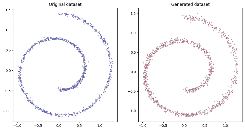
The results are not very different from what we plotted before, yet we obtained them in a fraction of the time. A better structure for the network (typically, a U-net) would have helped.
fig, (ax0, ax1) = plt.subplots(figsize=(12, 6), ncols=2)
n = 1_000
ax0.scatter(dataset[:n, 0], dataset[:n, 1], alpha=0.5, color='blue', edgecolor='grey', s=5)
ax0.set_title('Original dataset')
x_all = torch.stack(compute_reverse_process(model, n))
ax1.scatter(x_all[-1][:, 0], x_all[-1][:, 1], alpha=0.5, color='crimson', edgecolor='grey', s=5)
ax1.set_title('Generated dataset');
We conclude this post with a note for two good blogs in the subject: Lil’Lol post on the topic is one of the best introductions that can be found on the web, while Emilio Dorigatti post inspired the code for the first part of this post. Very noteworthy is also Calvin Luo paper on diffusion models; it contains most of the formulae presented in this post.