In this article we look at batch reinforcement learning. An agent has two main priorities: it must explore its environment effectively so as to obtain useful experiences, and it must learn effectively from these experiences. In online reinforcement learning, both challenges are attacked simultaneously, with numerous interactions between the gathering experience and the learning it (that is, the training of the deep neural networks). In offline reinforcement learning, instead, the two phases of data collection and the policy optimization are clearly decoupled. This situation arises often in settings where online experimentation is impossible or impractical: think of hard-to-obtain data, like medical treatment, emergency response, or the real-life behavior of some complicated robot you don’t want to destroy at any new exploration. Since in order to gather data you need a policy in the first place, the goal of offline learning is often to learn a policy that outperforms those used to generate the dataset of past experiences. Batch algorithms tend to be more data efficient and stable; they also generally ignore the exploration-exploitation problem, doing their best with the data they have.
A first example is the Least Square Policy Iteration (LSPI), which learns a linear approximation of the Q-function. The method is very stable, with not many hyperparameters that need tweaking. It is, however, limited to linear functions over a given set of features. An alternative are fitted Q-iterations, of which we consider a variant based on neural networks.
The algorithm is as follows:
- generate a batch of transitions \(\mathcal{D} = \left\{(s_i, a_i, r_i, s^\prime_i), i = 1, \ldots, N_{batch} \right\}\) for some fixed positive number $N_{batch}$;
- initialize an approximate Q-function $\hat{Q}_\theta$, in our case using deep neural networks, with parameters $\theta$;
- initialize the training set $\mathcal{T}$;
- for each $(s_i, a_i, r_i, s^\prime_i) \in \mathcal{D}$:
- compute \(\hat{q}_i = \gamma \max_{a^\prime} \hat{Q}_\theta (s^\prime_i, a_i);\)
- add the training sample $(s_i, a_i), \hat{q}_i$ to $\mathcal{T}$;
- learn $\hat{Q}_\theta$ from $\mathcal{T}$;
- go to step 3.
The DQN method we have used to solve the cart pole problem fits in this framework, with the additional trick of experience replay. What we will implement here is the other approach: get enough data to start with, using any policy (random in our case), the learn $\hat{Q}_\theta$ and use the resulting policy. This mean that we only go through steps 1 to 5 and ignore 6, even if that would be a simple addition. The method is easy to understand an implement, and can work well if the batch we collect is a reasonably complete representation of the environment.
We start with a few imports as usual.
import matplotlib.pylab as plt
import torch
from torch import nn
import torch.nn.functional as F
import random
import time
import copy
from collections import deque, namedtuple
import numpy as np
import gym
from tqdm.notebook import tnrange as trange

device = torch.device("cuda" if torch.cuda.is_available() else "cpu")
The environment is Acrobot-v0. Acrobot is a 2-link pendulum with only the second joint actuated.
Initially, both links point downwards. The goal is to swing the
end-effector at a height at least the length of one link above the base.
Both links can swing freely and can pass by each other, i.e., they don’t
collide when they have the same angle. The action is either applying -1, 0 or +1 torque on the joint between
the two pendulum links. This problem is not deterministic, as some noise is added to the effect of the torque.
It is a simple problem that can be solved without GPUs on a normal computer in a few minutes, which is quite good for experimenting.
env = gym.make('Acrobot-v1')
num_actions = env.action_space.n
print(f"Environment has {num_actions} actions")
Environment has 3 actions
As we have done before, we define a transition tuple. We also store a done field as this will make the subsequent code easier and faster.
Transition = namedtuple('Transition', ('state', 'action', 'next_state', 'reward', 'done'))
To easy the learning phase, we only keep episodes that have achieved something, discarding episodes whose total reward is close to -500. This isn’t needed and it ad-hoc for this environment.
num_episodes = 5_000

total_steps = []
total_rewards = []
data = []

for _ in trange(num_episodes):
    state, done, rewards = env.reset(), False, []
    tmp = []
    while not done:
        action = random.randint(0, num_actions - 1)
        next_state, reward, done, _ = env.step(action)
        tmp.append(Transition(state, np.array([action], dtype=np.int64), next_state, np.array([reward]), done))
        rewards.append(reward)
        state = next_state
    total_rewards.append(sum(rewards))
    total_steps.append(len(rewards))
    # keep only the episodes that have reached the goal
    if total_rewards[-1] > -475:
        data += tmp

print(f"Total number of collected transitions: {len(data)}")
Total number of collected transitions: 27290
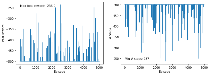
We visualize what we obtained over the five thousand episodes. A lot didn’t go anywhere (so the total reward is -500), yet we have several that worked in some sense, with a maximum total reward of about 250. The lenght of the episodes is the reverse of the total reward, as 500 iterations means the goal wasn’t reached.
fig, (ax0, ax1) = plt.subplots(figsize=(12, 4), ncols=2)
ax0.plot(total_rewards)
ax0.set_xlabel('Episode')
ax0.set_ylabel('Total Reward')
ax1.plot(total_steps)
ax1.set_xlabel('Episode')
ax1.set_ylabel('# Steps')
ax0.text(0, -245, f'Max total reward: {max(total_rewards)}')
ax1.text(0, 245, f'Min # steps: {min(total_steps)}');
This is the $\hat{Q}_\theta$ approximation using a simple neural network with ReLU activation function.
class Net(nn.Module):

    def __init__(self, input_shape, num_actions):
        super().__init__()
        self.linear1 = nn.Linear(input_shape, 32)
        self.linear2 = nn.Linear(32, 16)
        self.linear3 = nn.Linear(16, num_actions)

    def forward(self, x):
        x = torch.relu(self.linear1(x))
        x = torch.relu(self.linear2(x))
        x = self.linear3(x)
        return x
The DataSet class is a nice PyTorch utility that wraps our data and can then be passed to the DataLoader. This
allows us to easily sample the mini-batches that are needed by the optimizer.
class MyDataSet(torch.utils.data.Dataset):

    def __init__(self, transitions):
        super().__init__()
        self.transitions = transitions

    def __len__(self):
        return len(self.transitions)

    def __getitem__(self, idx):
        return self.transitions[idx]
net = Net(env.observation_space.shape[0], num_actions)
dataset = MyDataSet(data)
loader = torch.utils.data.DataLoader(dataset=dataset, batch_size=128, shuffle=True)
loss = nn.MSELoss()
optimizer = torch.optim.Adam(net.parameters(), lr=1e-2)
gamma = 0.95
This is the learning part: we iterate ove the mini-batches, compute the loss function, and iterate a few times.
num_epochs = 10
for epoch in range(num_epochs):
    total_diff = 0.0
    for state, action, next_state, reward, done in loader:
        lhs = net(state.float()).gather(1, action)
        rhs = reward.float()
        mask = [not k for k in done]
        rhs[mask] += gamma * net(next_state[mask].float()).max(1)[0].reshape(-1, 1)
        diff = loss(lhs, rhs)
        optimizer.zero_grad()
        diff.backward()
        optimizer.step()
        total_diff += diff.item()
    total_diff /= len(loader)
    print(f"Epoch: {epoch + 1}, average total diff = {total_diff}")
Epoch: 1, average total diff = 0.2936705021518413
Epoch: 2, average total diff = 0.20949850663124958
Epoch: 3, average total diff = 0.18696966070995152
Epoch: 4, average total diff = 0.17259137656226337
Epoch: 5, average total diff = 0.16138896105863224
Epoch: 6, average total diff = 0.1569221820508208
Epoch: 7, average total diff = 0.14005955475791593
Epoch: 8, average total diff = 0.12499631060478843
Epoch: 9, average total diff = 0.11886832563676566
Epoch: 10, average total diff = 0.11583108482795341
To test the policy we run over 100 episodes and compute the total reward. The average is around -100, which is more than the best result we go in the training set! The agent has learned how to generalize from the training set to the particular cases seen in the testing.
total_rewards = []
for _ in range(100):
    state, done, total_reward = env.reset(), False, 0.0
    while not done:
        action = net(torch.tensor([state], dtype=torch.float)).max(1)[1].item()
        next_state, reward, done, _ = env.step(action)
        total_reward += reward
        state = next_state
    total_rewards.append(total_reward)
plt.plot(total_rewards)
avg = sum(total_rewards) / len(total_rewards)
plt.title(f'Average reward: {avg}')
plt.xlabel('Testing Episode')
plt.ylabel('Total Reward');
plt.axhline(y=avg, linestyle='dashed', color='red')
<matplotlib.lines.Line2D at 0x245180179d0>
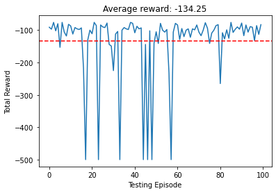
The results aren’t always great, but we have not used too many transitions, and we have only generated one batch. To see better results we should generate a few batches, using the policy coming from the previous $\hat{Q}_\theta$. To finish the article, we generate a small video.
from PIL import Image, ImageDraw, ImageFont

state, done = env.reset(), False
frames = [env.render(mode='rgb_array')]
rewards = []
while not done:
    action = net(torch.tensor([state], dtype=torch.float)).max(1)[1].item()
    next_state, reward, done, _ = env.step(action)
    rewards.append(reward)
    frame = env.render(mode='rgb_array')
    image = Image.fromarray(frame)
    draw = ImageDraw.Draw(image)
    font = ImageFont.truetype("font3270.otf ", 24)
    text = f"Step # {len(frames)}\n"
    if action == 0:
        action_as_str = 'negative torque'
    elif action == 1:
        action_as_str = 'no torque'
    else:
        action_as_str = 'positive torque'
    text += f"action: {action_as_str}\n"
    text += f"total reward: {sum(rewards)}"
    draw.multiline_text((10, 10), text, fill=128, font=font)
    frames.append(np.array(image))
    state = next_state
# add the last image a few more times for a nicer gif
for _ in range(20):
    frames.append(frames[-1])
print(f"Total reward: {sum(rewards)}, # steps = {len(rewards)}")
Total reward: -98.0, # steps = 99
from matplotlib import pyplot as plt
from matplotlib import animation

# np array with shape (frames, height, width, channels)
video = np.array(frames[:])

fig = plt.figure(figsize=(8, 6))
im = plt.imshow(video[0,:,:,:])
plt.axis('off')
plt.close() # this is required to not display the generated image

def init():
    im.set_data(video[0,:,:,:])

def animate(i):
    im.set_data(video[i,:,:,:])
    return im

anim = animation.FuncAnimation(fig, animate, init_func=init, frames=video.shape[0],
                               interval=100)
anim.save('./acrobot-video.gif')

The advantage of this approach is that the learning phase is well-defined and stable; the disadvantage is that we must get meaningful transitions in our batch to learn a useful policy.