In the previous article we looked at how autoencoders work. As we noticed, in general the latent space is a non-convex manifold and the latent variables have arbitrary scales. This makes basic autoencoders a poor choice for generative models. Variational autoencoders fix this issue by ensuring that the latent variables follows a desirable distribution from which we can easily sample from.
Variational autoencoders were introduced by Kingma and Welling. Their derivation of variational autoencoers is substantially more involved than that of autoencoeders. We assume that the each observation variables $x$ is a sample from an unknown underlying process, whose true distribution $p^\star(x)$ is unknown. We attempt to approximate this process with a chosen model with parameters $\theta$,
\[x \sim p_\theta(x),\]with the goal of finding $\theta$ such that
\[p_\theta(x) \approx p^\star(x).\]The first step is to extend our model to include latent variables – that is, variables that are part of our model but we don’t observe, and therefore are not explicitly present in our dataset. These variables are denoted as $z$, with $p(x, z)$ the joint distribution over the observation variables $x$ and the latent variables $z$. The marginal distribution over the observation variables $p_\theta(x)$ is
\[p_\theta(x) = \int p_\theta(x, z) dz.\]Such implicit distribution over $z$ can be quite flexible; this expressivity makes it attractive for approximating complicated underlying distributions $p^\star(x)$. We will write
\[p_\theta(x, z) = p_\theta(x \vert z) p_\theta(z),\]where both $p_\theta(x\vert z)$ and $p_\theta(z)$ will be specified by us.
Since $p_\theta(z)$ is not conditioned on any observation, it is called the prior. Once $p_\theta(z)$ and $p_\theta(x\vert z)$ are defined, we would use maximum likelyhood to define the model parameters $\theta$. More precisely, we will maximize $\log p_\theta(x)$. We also introduce a distribution $q_\phi(z\vert x)$, depending on some parameters $\phi$ to be optimized as well, which we will define later on.
We have:
\[\begin{aligned} \log p_\theta(x) & = \log \int p_\theta(x | z) p_\theta(z) dz \\ % & = \log \int p_\theta(x | z) \frac{q_\phi(z | x)}{q_\phi(z | x)} p_\theta(z) dz \\ % & \ge \int \log \left[ \frac{p_\theta(z)}{q_\phi(z | x)} p_\theta(x | z) \right] q_\phi(z | x) dz \\ % & = \underbrace{\mathbb{E}_{q_\phi(z | x)} \left[ \log{\frac{p_\theta(z)}{q_\phi(z | x)} } \right]}_{(A)} + \underbrace{\mathbb{E}_{q_\phi(z | x)}\left[ \log p_\theta(x | z) \right]}_{(B)}, \end{aligned}\]where the inequality is a consequence of Jensen’s inequality.
Let’s look at the (B) first. We assume a Gaussian observation model, that is
\[p_\theta(x | z) \sim \mathcal{N}(x; D_\theta(z), \eta I),\]that is each term $x$ is obtained from a Gaussian distribution with mean $D_\theta(z)$, acting on the latent variables $z$, and variance $\eta$, with $I$ the identity matrix whose size equals the dimension of the latent space $m$. The function $D_\theta(z)$ is called the decoder, as it converts the latest space into the observation space. Because of our choice, we have
\[\begin{aligned} \log p_\theta(x | z) & = \log \mathcal{N}(x; D_\theta(\zeta), \eta I) \\ % & = \log \left[ \frac{1}{\left( 2 \pi \eta \right)^{m / 2}} \exp\left( - \frac{1}{2 \eta} \|x - D_\theta(z) \|^2 \right) \right] \\ % & = -\frac{1}{2 \eta} \|x - D_\theta(z) \|^2 + const, \end{aligned}\]to be evaluated on $q_\phi(z\vert x)$ using a Monte Carlo approximation.
Term (A) is
\[\begin{aligned} \mathbb{E}_{q_\phi(z | x)} \left[ \log \frac{p_\theta(z)}{ q_\phi(z | x)} \right] & = \int \left[ \log p_\theta(z) - \log q_\phi(z | x) \right] dq_\phi(z | x) \\ % & = - D_{KL}(q_\phi(z | x) || p_\theta(z)). \end{aligned}\]The Kullback-Leibler divergence term $D_{KL}$ is widely used as a measure of probability distance (though it doesn’t satisfy the axioms to be a distance metric); as part of our optimization procedure, it will encourage $q_\phi(z \vert x)$ to be as close as possible to $p_\theta(z)$, which we model as
\[p_\theta(z) \sim \mathcal{N}(0, I).\]we still need to define a model for $q_\phi(z \vert x)$. Sticking to our Gaussian mixtures, we take
\[q_\phi(z | x) \sim \mathcal{N}(z; \mu_\phi(x), \Sigma_\phi(x)),\]where $\mu_\phi(x)$ and $\Sigma_\phi(x)$ are the mean and the variance of the distribution, and the output of a neural network with parameters $\phi$ and acting on $E_\phi(x)$, where $E_\phi(x)$ is another neural network, called the $encoder$, that acts on the observations. By notation we define the vector $\mu_\phi(x)$ to be
\[\mu_\phi(x) = (\mu_{\phi, 1}(x), \ldots, \mu_{\phi, m} (x))\]and we take to covariance matrix as
\[\Sigma_\phi(x) = diag (\sigma^2_{\phi, 1}(x), \ldots, \sigma^2_{\phi, m}(x)).\]Because of this choice, the KL divergence can be computed explicitly,
\[\begin{aligned} D_{KL} & = \int \log \frac{q_\phi(z | x)}{p_\theta(z)} q_\phi(z | x) dz \\ % & = \int \left[ \log q_\phi(z | x) - \log p_\theta(z) \right] q_\phi(z | x) dz \\ % & = \int \left[ \log \Pi_i \frac{1}{\sigma_{\phi,i} \sqrt{2 \pi}} \exp \left( -\frac{1}{2} \left( \frac{z - \mu_{\phi, i}(x)}{\sigma_{\phi, i}(x)} \right)^2 \right) - \log \Pi_i \frac{1}{\sqrt{2 \pi}} \exp \left( -\frac{z^2}{2} \right) \right] \\ % & \quad \quad \times \Pi_i \frac{1}{\sigma_{\phi,i} \sqrt{2 \pi}} \exp \left( -\frac{1}{2} \left( \frac{z - \mu_{\phi, i}(x)}{\sigma_{\phi, i}(x)} \right)^2 \right) dz \\ % & = \sum_i \int \left( \log \frac{1}{\sigma_{\phi, i}} - \frac{1}{2} \left( \frac{z - \mu_{\phi, i}}{\sigma_{\phi, i}} \right)^2 + \frac{1}{2} z^2 \right) \frac{1}{\sigma_{\phi,i} \sqrt{2 \pi}} \\ % & \quad \quad \times \exp \left( -\frac{1}{2} \left( \frac{z - \mu_{\phi, i}(x)}{\sigma_{\phi, i}(x)} \right)^2 \right) dz \\ % & = \sum_i \left( \log \frac{1}{\sigma_{\phi, i}(x)} - \frac{1}{2} + \frac{1}{2} \left( \sigma_{\phi, i}^2 + \mu_{\phi, i}^2 \right) \right) \\ % & = \sum_i \frac{1}{2} \left( \sigma_{\phi, i}^2 + \mu_{\phi, i}^2 - 1 - \log \sigma_{\phi, i}(x)^2 \right). \end{aligned}\]There is still an issue to be solved: to apply $p_\theta(x \vert z)$ and $q_\phi(z \vert x)$, we need to draw random number from the corresponding probability distributions. In general it is difficult to differentiate in such cases, but since we have selected Gaussian variates we can use the reparametrization trick. For example to apply $q_\phi(z \vert x)$ we would have
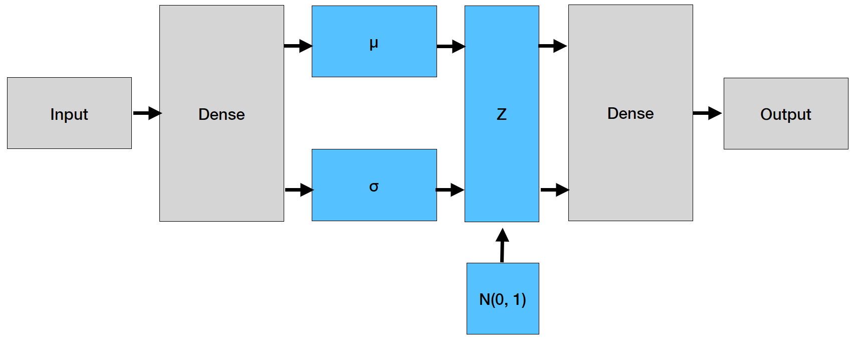
\[z_i = \mu_i + \epsilon_i \sigma_i,\]where $\epsilon_i \sim \mathcal{N}(0, 1)$, while $\mu_i$ and $\sigma_i$ are the output of the neural network.
The architecture is reported in the picture below. Note that the dense layer is connected to two separate blocks, one of which generates $\mu$ and the other $\sigma$. The part is the encoder. Once $Z$ has been generated, we enter the decoder that rebuilds the inputs from the encodings.
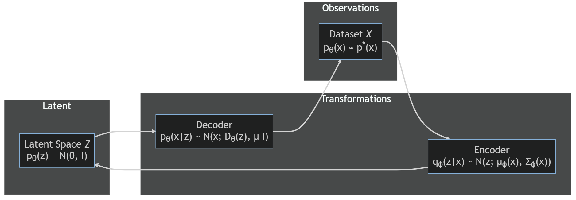
The implementation is quite close to that of an autoencoder; the differences are in the final part of the encoder, with application of the $\mu_\phi$ and $\sigma_\phi$ to the output of $E_\phi(x)$, and the loss function, which contains the two terms we have been above. The diagram below shows the different assumptions on the probability distributions.
from matplotlib.patches import Circle
import matplotlib.pyplot as plt
import numpy as np
from scipy.optimize import minimize
import seaborn as sns
import torch
import torch.nn as nn
import torch.nn.functional as F
import torch.utils
import torch.distributions
from torch.utils.data import Dataset, DataLoader
device = 'cpu' # if torch.cuda.is_available() else 'cpu'
num_inputs = 10_000
num_points = 100
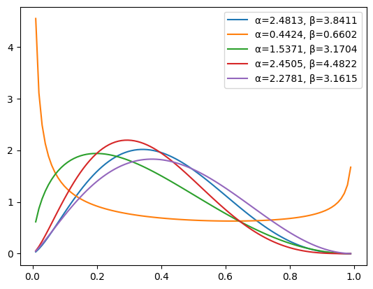
To test the method, we build a dataset that is composed by the sampling on a uniform grid of the probability density function of the beta distribution, for some values of the parameters $\alpha$ and $\beta$. In particular, we look at $\alpha \in [0, 5], \beta in [0, 5]$. Ideally, the final variational autoencoder will be capable of generating distributions that look reasonable in that class.
uniform_dist = torch.distributions.uniform.Uniform(0, 5)
grid = torch.linspace(0.01, 0.99, num_points)
def target_func(grid, α, β):
    # return the log of the probability, not the probability itself
    return torch.distributions.Beta(α, β).log_prob(grid)
The generation of the dataset is in a simple loop. For simplicity we don’t define a training and a test dataset.
torch.manual_seed(0)
X, Y = [], []
for _ in range(num_inputs):
    α = uniform_dist.sample()
    β = uniform_dist.sample()
    X.append(target_func(grid, α, β))
    Y.append([α, β])
X = torch.vstack(X)

assert X.shape[0] == num_inputs
assert X.shape[1] == num_points
assert X.isnan().sum() == 0.0
We plot the first 5 entries of the dataset, seeing – as expected – that the shapes can be quite different.
for x, (α, β) in zip(X[:5], Y[:5]):
    plt.plot(grid, x.exp(), label=f'α={α.item():.4f}, β={β.item():.4f}')
plt.legend()
<matplotlib.legend.Legend at 0x16e68326b80>
normal_dist = torch.distributions.Normal(0, 1)
if device == 'cuda':
    normal_dist.loc = normal_dist.loc.cuda()  # hack to get sampling on the GPU
    normal_dist.scale = normal_dist.scale.cuda()
The encoder is a bit different from the corresponding one for non-variational autoencoders, but not by much. The definition of $E_\phi(x)$ is indeed the same, however it is followed by the application of the $\mu_\phi$ and $\Sigma_\phi$ and the computation of the KL divergence. Codewise, though, it is a small change.
class VariationalEncoder(nn.Module):

    def __init__(self, latent_dims, num_hidden):
        super().__init__()
        self.linear1 = nn.Linear(num_points, num_hidden)
        self.linear2 = nn.Linear(num_hidden, num_hidden)
        self.linear3 = nn.Linear(num_hidden, num_hidden)
        self.linear_mu = nn.Linear(num_hidden, latent_dims)
        self.linear_logsigma2 = nn.Linear(num_hidden, latent_dims)

    def forward(self, x):
        x = torch.tanh(self.linear1(x))
        x = torch.tanh(self.linear2(x))
        x = torch.tanh(self.linear3(x))
        mu =  self.linear_mu(x)
        logsigma2 = self.linear_logsigma2(x)
        sigma = torch.exp(logsigma2 / 2)
        z = mu + sigma * normal_dist.sample(mu.shape)
        integrand = (sigma**2 + mu**2 - logsigma2 - torch.ones_like(sigma)) / 2
        kl = torch.mean(torch.sum(integrand, axis=1), axis=0)
        return z, kl
The decoder is instead the same.
class Decoder(nn.Module):

    def __init__(self, latent_dims, num_hidden):
        super(Decoder, self).__init__()
        self.linear1 = nn.Linear(latent_dims, num_hidden)
        self.linear2 = nn.Linear(num_hidden, num_hidden)
        self.linear3 = nn.Linear(num_hidden, num_hidden)
        self.linear4 = nn.Linear(num_hidden, num_points)

    def forward(self, z):
        z = torch.tanh(self.linear1(z))
        z = torch.tanh(self.linear2(z))
        z = torch.tanh(self.linear3(z))
        return self.linear4(z)
The variational autoencoder is simply the composition of the encoder and the decoder, exactly as it was for the non-variational case. There are two small differences: the forward() method returns the KL divergence as well, and we have a method to compute the term (B) with the appropriate scaling by $\eta$ and the reparametrization trick. Sometimes the scaling $\eta$ is omitted; here we keep it.
class VariationalAutoencoder(nn.Module):

    def __init__(self, latent_dims, num_hidden):
        super().__init__()
        self.encoder = VariationalEncoder(latent_dims, num_hidden)
        self.decoder = Decoder(latent_dims, num_hidden)

    def forward(self, x):
        z, kl = self.encoder(x)
        x_hat = self.decoder(z)
        return x_hat, kl

    def compute_log_likelihood(self, X, X_hat, η):
        ξ = normal_dist.sample(X_hat.shape)
        X_sampled = X_hat + η.sqrt() * ξ
        return 0.5 * F.mse_loss(X, X_sampled) / η #+ η.log()
def init_weights(m):
    if isinstance(m, nn.Linear):
        torch.nn.init.xavier_uniform_(m.weight)
        m.bias.data.fill_(0.01)
To use the DataLoader we define a simple customization of the Dataset class.
class FuncDataset(Dataset):

    def __init__(self, X):
        self.X = X

    def __len__(self):
        return len(self.X)

    def __getitem__(self, idx):
        return self.X[idx]
data_loader = DataLoader(FuncDataset(X), batch_size=32, shuffle=True)
We are ready for the training, which is almost identical to the non-variational part. The optimizer doesn’t seem to make much of a difference.
def train(vae, data, epochs, lr, gamma, η, β, print_every):
    η = torch.tensor(η)
    optimizer = torch.optim.Adam(vae.parameters(), lr=lr)
    scheduler = torch.optim.lr_scheduler.ExponentialLR(optimizer, gamma=gamma)
    history = []
    for epoch in range(epochs):
        last_lr = scheduler.get_last_lr()
        total_log_loss, total_kl_loss, total_loss = 0.0, 0.0, 0.0
        for x in data:
            x = x.to(device)  # GPU
            optimizer.zero_grad()
            x_hat, kl_loss = vae(x)
            log_loss = vae.compute_log_likelihood(x, x_hat, η)
            loss = log_loss + β * kl_loss
            total_log_loss += log_loss.item()
            total_kl_loss += kl_loss.item()
            total_loss += loss.item()
            loss.backward()
            optimizer.step()
        scheduler.step()
        if (epoch + 1) % print_every == 0:
            print(f"Epoch: {epoch + 1:3d}, lr: {last_lr[0]:.4e}, " \
                  f"total log loss: {total_log_loss:.4f}, total KL loss: {total_kl_loss:.4f}, " \
                  f"total loss: {total_loss:.4e}")
        history.append((total_log_loss, total_kl_loss))
    return np.array(history)
torch.manual_seed(0)
data_loader = DataLoader(FuncDataset(X), batch_size=256, shuffle=True)
latent_dims = 2
vae = VariationalAutoencoder(latent_dims, num_hidden=32).to(device)
vae.apply(init_weights)
history = train(vae, data_loader, epochs=1_000, lr=1e-3, gamma=0.99, η=0.1**2, β=1, print_every=50)
Epoch:  50, lr: 6.1112e-04, total log loss: 172.4695, total KL loss: 216.1071, total loss: 3.8858e+02
Epoch: 100, lr: 3.6973e-04, total log loss: 87.6573, total KL loss: 210.6503, total loss: 2.9831e+02
Epoch: 150, lr: 2.2369e-04, total log loss: 73.5103, total KL loss: 209.3993, total loss: 2.8291e+02
Epoch: 200, lr: 1.3533e-04, total log loss: 69.3126, total KL loss: 208.9647, total loss: 2.7828e+02
Epoch: 250, lr: 8.1877e-05, total log loss: 66.7518, total KL loss: 210.3983, total loss: 2.7715e+02
Epoch: 300, lr: 4.9536e-05, total log loss: 65.2317, total KL loss: 208.2934, total loss: 2.7353e+02
Epoch: 350, lr: 2.9970e-05, total log loss: 65.0135, total KL loss: 208.5284, total loss: 2.7354e+02
Epoch: 400, lr: 1.8132e-05, total log loss: 64.8618, total KL loss: 208.3012, total loss: 2.7316e+02
Epoch: 450, lr: 1.0970e-05, total log loss: 65.0291, total KL loss: 208.7231, total loss: 2.7375e+02
Epoch: 500, lr: 6.6369e-06, total log loss: 64.8451, total KL loss: 208.4879, total loss: 2.7333e+02
Epoch: 550, lr: 4.0153e-06, total log loss: 64.3602, total KL loss: 208.6472, total loss: 2.7301e+02
Epoch: 600, lr: 2.4293e-06, total log loss: 63.9771, total KL loss: 208.3997, total loss: 2.7238e+02
Epoch: 650, lr: 1.4697e-06, total log loss: 64.4275, total KL loss: 208.3166, total loss: 2.7274e+02
Epoch: 700, lr: 8.8920e-07, total log loss: 64.6008, total KL loss: 208.7841, total loss: 2.7338e+02
Epoch: 750, lr: 5.3797e-07, total log loss: 64.3160, total KL loss: 208.5707, total loss: 2.7289e+02
Epoch: 800, lr: 3.2548e-07, total log loss: 63.8710, total KL loss: 208.4223, total loss: 2.7229e+02
Epoch: 850, lr: 1.9692e-07, total log loss: 64.5717, total KL loss: 208.6061, total loss: 2.7318e+02
Epoch: 900, lr: 1.1914e-07, total log loss: 63.6378, total KL loss: 207.9878, total loss: 2.7163e+02
Epoch: 950, lr: 7.2077e-08, total log loss: 64.7554, total KL loss: 208.2642, total loss: 2.7302e+02
Epoch: 1000, lr: 4.3607e-08, total log loss: 63.8177, total KL loss: 208.0312, total loss: 2.7185e+02
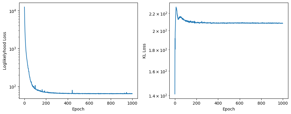
fig, (ax0, ax1) = plt.subplots(figsize=(10, 4), ncols=2)
ax0.semilogy(history[:, 0])
ax0.set_xlabel('Epoch')
ax0.set_ylabel('Loglikelyhood Loss')
ax1.semilogy(history[:, 1])
ax1.set_xlabel('Epoch')
ax1.set_ylabel('KL Loss')
fig.tight_layout()
The first thing we do is to apply the encoder to the entire dataset and check the distribution of the latent variables.
Z = []
for entry in X:
    Z.append(vae.encoder(entry.unsqueeze(0).to(device))[0].cpu().detach().numpy().squeeze(0))
Z = np.array(Z)
fig, (ax0, ax1, ax2) = plt.subplots(figsize=(12, 4), ncols=3)
sns.histplot(Z[:, 0], ax=ax0, stat='density')
sns.histplot(Z[:, 1], ax=ax1, stat='density')
ax2.scatter(Z[:, 0], Z[:, 1], color='salmon')
ax0.set_xlabel('$z_1$')
ax1.set_xlabel('$z_2$')
ax2.set_xlabel('$z_1$'); ax2.set_ylabel('$z_2$')
for r in [1, 2, 3, 4, 5]:
    ax2.add_patch(Circle((0, 0), r, linestyle='dashed', color='crimson', alpha=1, fill=None))
fig.tight_layout()
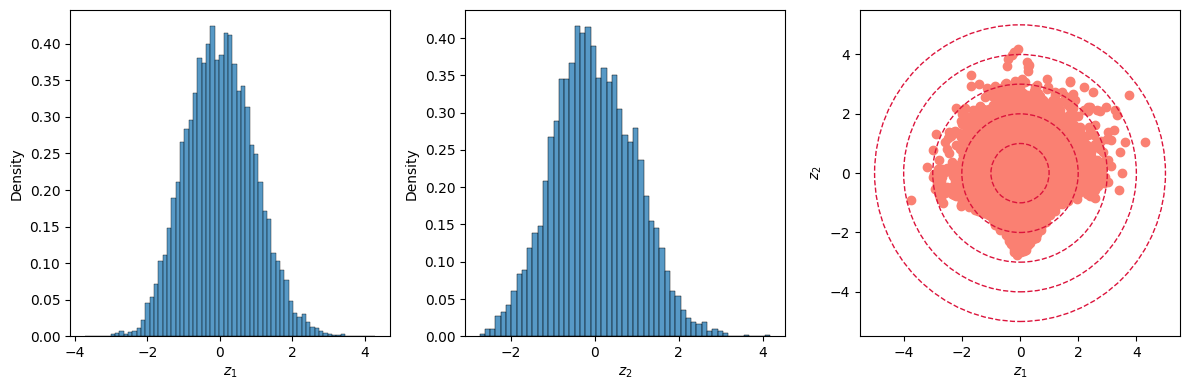
Both latent dimensions $Z_1$ and $Z_2$ have a distribution resembling the one of a normal variate; their joint distribution is nicely scattered around the origin are roughtly within 3 to 4 standard deviations, as the red circles (with a radius of 1, 2, 3 and 4, respectively) show.
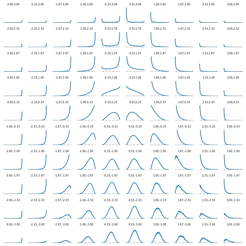
As an example of what each latent variable represents we plot, on a 10 by 10 grid, the result of the decoder for several values of $z_1$ and $z_2$, both ranging from -1 to 1, where can see the shape of the Beta distributions changing with the two parameters as we would expect. The dotted grey line indicates the zero axis; all plots share the same scale on the Y axis.
n = 10
fig, axes = plt.subplots(nrows=n, ncols=n, figsize=(8, 8), sharex=True, sharey=True)
for i, z_1 in enumerate(np.linspace(-3, 3, n)):
    for j, z_2 in enumerate(np.linspace(-3, 3, n)):
        y = vae.decoder(torch.FloatTensor([z_1, z_2]).to(device)).detach().cpu().exp()
        axes[n - 1 - j, i].plot(grid, y)
        axes[n - 1 - j, i].plot(grid, np.zeros_like(grid), color='grey', linestyle='dashed')
        axes[n - 1 - j, i].axis('off')
        axes[n - 1 - j, i].set_title(f'{z_1:.2f},{z_2:.2f}', fontsize=6)
        axes[n - 1 - j, i].set_ylim(0, 3)
fig.tight_layout()
Because of the distribution of the latent variables, it is then much easier to generate new values or look for the optimal ones that match a given, which is what we try now to do. First, we generate two random values for $\alpha$ and $\beta$ and compute the corresponding exact PDF; then we use scipy to find the values of $(Z_1, Z_2)$ that produce the closest match.
α = uniform_dist.sample()
β = uniform_dist.sample()

print(f'Params for the test: α={α.item():.4f}, β={β.item():.4f}')

X_target = target_func(grid, α, β).numpy()

def func(x):
    X_pred = vae.decoder(torch.FloatTensor(x).to(device))
    X_pred = X_pred.cpu().detach().numpy()
    diff = np.linalg.norm(X_target - X_pred).item()
    return diff

res = minimize(func, [0.0, 0.0], method='Nelder-Mead')
res
Params for the test: α=3.4180, β=0.2701


       message: Optimization terminated successfully.
       success: True
        status: 0
           fun: 0.26235488057136536
             x: [-1.498e+00  6.091e-01]
           nit: 69
          nfev: 132
 final_simplex: (array([[-1.498e+00,  6.091e-01],
                       [-1.498e+00,  6.091e-01],
                       [-1.498e+00,  6.091e-01]]), array([ 2.624e-01,  2.624e-01,  2.624e-01]))
X_pred = vae.decoder(torch.FloatTensor(res.x).to(device)).cpu().detach().numpy()
fig, (ax0, ax1) = plt.subplots(figsize=(10, 4), ncols=2)
ax0.plot(grid, np.exp(X_target), label=f'α={α.item():.4f}, β={β.item():.4f}')
ax0.plot(grid, np.exp(X_pred), label=f'$z_1$={res.x[0].item():.4f}, $z_2$={res.x[1].item():.4f}')
ax0.legend()
ax1.plot(grid, np.exp(X_target) - np.exp(X_pred))
ax0.set_xlabel('x')
ax0.set_ylabel('β(x; α, β)')
ax0.set_title('PDF')
ax1.set_xlabel('x')
ax1.set_title('Error')
ax1.set_ylabel('$β(x; α, β) - \hat{β}(x; z_1, z_2)$')
fig.tight_layout()
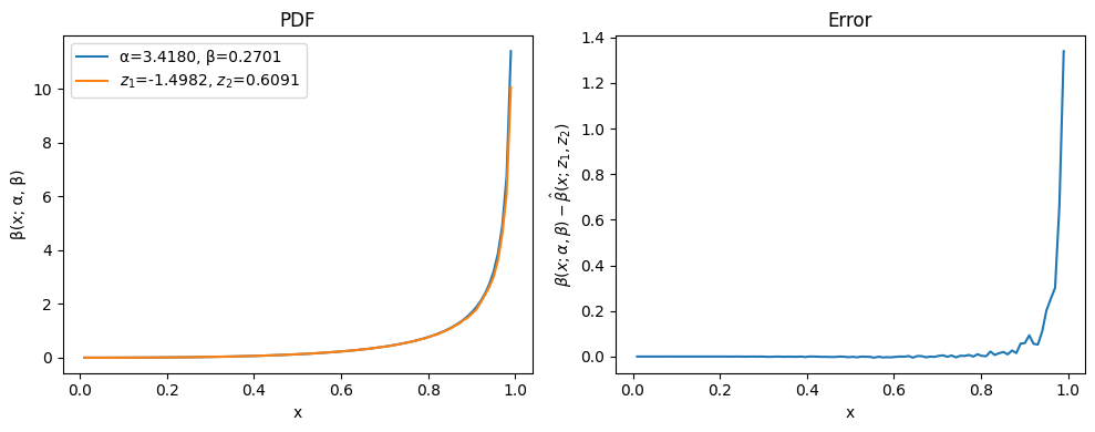
The results isn’t too bad – true, the reconstructed curve oscillates a bit, but at a small scale. the oscillations can be resolved with more training data and more iterations, or by increasing the size of the neural networks. We can say that the encoder has managed to compress the input data to two parameters and the decoder to define how to build the PDF of the beta distribution from those.