In this article we continue the exploration of functional principal component analysis (FPCA) that we did before. We start with a deeper look into Mercer’s theorem. The theorem states that every continuous, symmetric positive-definite function $K(x, y) : \Omega \times \Omega \rightarrow \mathbb{R}$, with $\Omega \in \mathbb{R}^d$, can be expressed as an infinite sum of product functions,
\[K(x, y) = \sum_{\ell=1}^\infty \lambda_\ell \varphi_\ell(x) \varphi_\ell(y),\]where the $\lambda_\ell$ are non-negative eigenvalues and the $\varphi_\ell$ the corresponding eigenfunctions. The convergence is absolute and uniform. This extends a classical result on symmetric positive-definite matrices to real fuctions.
Our interest of the above theorem is for functions $K(x, y)$ that are kernel functions. A Kernel function is a function that is symmetric, $K(x, y) = K(y, x), \forall x, y \in \Omega$, and is positive definite, meaning that for any finite set of points ${x_1, x_2, \ldots, x_d }$ and any real numbers ${ c_1, c_2, \ldots, c_n }$, the inequality \(\sum_{i, j} c_i c_j K(x_i, x_j) \ge 0\) holds. This means that the Gram matrix $G \in \mathbb{R}^{d \times d}$ with elements $G_{i, j} = K(x_i, x_j)$ is symmetric positive definite.
Common examples of kernel functions are, $\forall x, y \in \Omega = \mathbb{R}^d$,
- the linear kernel $K(x, y) = x^T y$,
- the polynomial kernel $K(x, y) = (x^T y + c)^n$, with $c \ge 0, n\ge 1$,
- the Gaussian kernel $K(x, y) = e^{ -\frac{\lVert x - y\rVert^2}{2 \sigma^2} }, \sigma > 0$, and
- the Laplacian kernel $K(x, y) = e^{-\alpha \lVert x - y \rVert}, \alpha > 0$.
As a simple example, we look at $\Omega = [a, b] \subset \mathbb{R}$ and $K(x, y) = f(x) f(y)$ for a generic function $f$. An eigenfunction $\varphi(x)$ must satisfy
\[\begin{aligned} \int_a^b K(x, y) \varphi(y) dy & = \lambda \varphi(x) \\ % \int_a^b f(x) f(y) \varphi(y) dy & = \lambda \varphi(x) \\ % f(x) \int_a^b f(y)\varphi(y) dy & = \lambda \varphi(x). \end{aligned}\]Assuming $\lambda \neq 0$, we must have $\varphi(x) = \alpha f(x)$ for some $x \in \mathbb{R}$, and consequently
\[f(x) \int_a^b f(y) \alpha f(y) dy = \lambda \alpha f(x)\]which yields
\[\lambda = \int_a^b f(y)^2 dy.\]To get the normalized eigenfunctions, we need
\[\int_a^b \alpha^2 f(y)^2 dy = 1,\]that is \(\alpha = \left( \int_a^b f(y)^2 dy \right)^{-1/2}.\)
It also follows that
\[\begin{aligned} \lambda \varphi(x) \varphi(y) & = \lambda \lambda^{-1/2} f(x) \lambda^{-1/2} f(y) \\ & = f(x) f(y) \\ & = K(x, y), \end{aligned}\]as expected from Mercer’s theorem, since there is only one eigenvalue (and eigenfunction).
In the case $f(x) = x$, it is easy to see that
\[\lambda = \int_a^b y^2 dy = \frac{1}{3}(b-a)^3\]and
\[\alpha = \left( \int_a^b y^2 dy \right)^{-1/2} = \lambda^{-1/2}.\]Therefore, \(\varphi(x) = \lambda^{-1/2} x.\)
After this small detour on Mercer’s theorem, we go back to the Karhunen-Loève Decomposition introduced in the previous article, focusing on two-dimensional problems, that is $d=2$. With a slight change of notation, we use $(x, y)$ to indicate a point in $\Omega = \mathbb{R}^2.$ We consider a sequence \(\{ V_t, t=1, \ldots, T\},\) where each $V_t$ is a sample of an unknown function $V(t, x, y)$, that is given a set of sampling points \(\{x_i, y_i, i=1, \ldots, I \},\) we have \(V_t = \{V_{t, i} = V(t, x_i, y_i), i=1, \ldots, I\}.\) For simplicity we consider $(x, y) \in \Omega = [-1, 1] \times [-1, 1]$, assuming that different domains can be mapped to $\Omega$.
The covariance operator $C(x, y, u, v)$ of the process \(\{V_t\}\), with $(x, y), (u, v) \in \Omega$, is a kernel operator in the sense defined above, and therefore we can apply Mercer’s theorem to it to identify the most important modes of such covariance operator. This means that we will identify a set of functions \(\{\varphi_\ell(x, y) : \Omega \rightarrow \mathbb{R}, \ell=1,\ldots, L\}\) that explain most of the variance in the process. To do this numerically, we proceed in two steps:
- we approximate $C$ numerically from the finite sequence \(\{V_t, t=1,\ldots, T\}\), and
- we define a finite-dimensional space that contains the functions $\varphi_\ell$.
Let’s focus first on the second step as for the first one we’ll do something quite simple. We will indicate with \(\{ \psi_b(x, y) : \Omega \rightarrow \mathbb{R}, b=1\, \ldots, B \}\) the set of basis functions of such space and operate exclusively in this space.
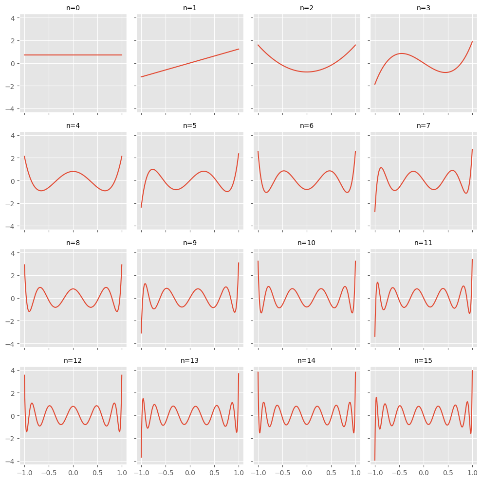
The basis functions we will use are Legendre polynomials, because this has certain advantages for our procedure, as we will see later on. Normalized Legendre polynomials of order $m$ are polynomials in the form
\[\mathcal{L}_m(x) = \frac{\sqrt{2m + 1}}{2} \frac{1}{2^m m!} \frac{d^m}{dx^m (x^2 - 1)^m}\]that are orthogonal in the sense that
\[\int_{-1}^1 \mathcal{L}_i(x) \mathcal{L}_j(x) dx = \delta_{ij},\]with $\delta_{ij}$ the Kronecher delta. Let’s visualize those polynomials.
import matplotlib.pyplot as plt
plt.style.use('ggplot')
import numpy as np
from scipy.special import eval_legendre
X = np.linspace(-1, 1)
fig, axes = plt.subplots(figsize=(10, 10), nrows=4, ncols=4, sharex=True, sharey=True)
axes = axes.flatten()
for n, ax in zip(range(0, 16), axes):
    y = eval_legendre(n, X) * np.sqrt((2 * n + 1 ) /2)
    ax.plot(X, y, label=r'$P_{}(x)$'.format(n))
    ax.set_title(f'n={n}', fontdict=dict(size=10))
fig.tight_layout()
To create basis functions for our two-dimensional case, we take the products of the first $n$ Legendre polynomials, such that the powers sums to at most $m$, with the first polynomial applied to $x$ and the second to $y$. Specifically, the basis functions $\psi_b(x, y), b=0, \ldots, B$ are defined as
\[\begin{aligned} \psi_1(x, y) & = \mathcal{L}_0(x) \mathcal{L}_0(y) \\ \psi_2(x, y) & = \mathcal{L}_1(x) \mathcal{L}_0(y) \\ \psi_3(x, y) & = \mathcal{L}_0(x) \mathcal{L}_1(y) \end{aligned}\]and so on. This gives a total of $B=\frac{1}{2}(n + 1)(n + 2)$ basis functions for any value of $m$. Because of the orthogonality discussed above, we have
\[\int_{-1}^1 \int_{-1}^1 \psi_i(x, y) \psi_j(x, y) dx dy = \delta_{i, j}.\]It is worthwhile to visualize those basis functions and appreciate their lack of smoothness as $m$ increases.
func2d = lambda x, y, i, j: eval_legendre(i, x) / np.sqrt(2 / (2 * i + 1)) * eval_legendre(j,y) / np.sqrt( 2 / (2 * j + 1))
n = 101
x = np.linspace(-1, 1, n)
y = np.linspace(-1, 1, n)
xx, yy = np.meshgrid(x, y)
fig = plt.figure(figsize=(20, 20))
counter = 0
m = 8
for i in range(m):
    for j in range(m):
        ax = fig.add_subplot(m, m, counter + 1, projection='3d')
        counter += 1
        zz = func2d(xx.flatten(), yy.flatten(), i, j).reshape(n, n)
        ax.plot_surface(xx, yy, zz, linewidth=0, antialiased=True)
        ax.axis('off')
fig.tight_layout()
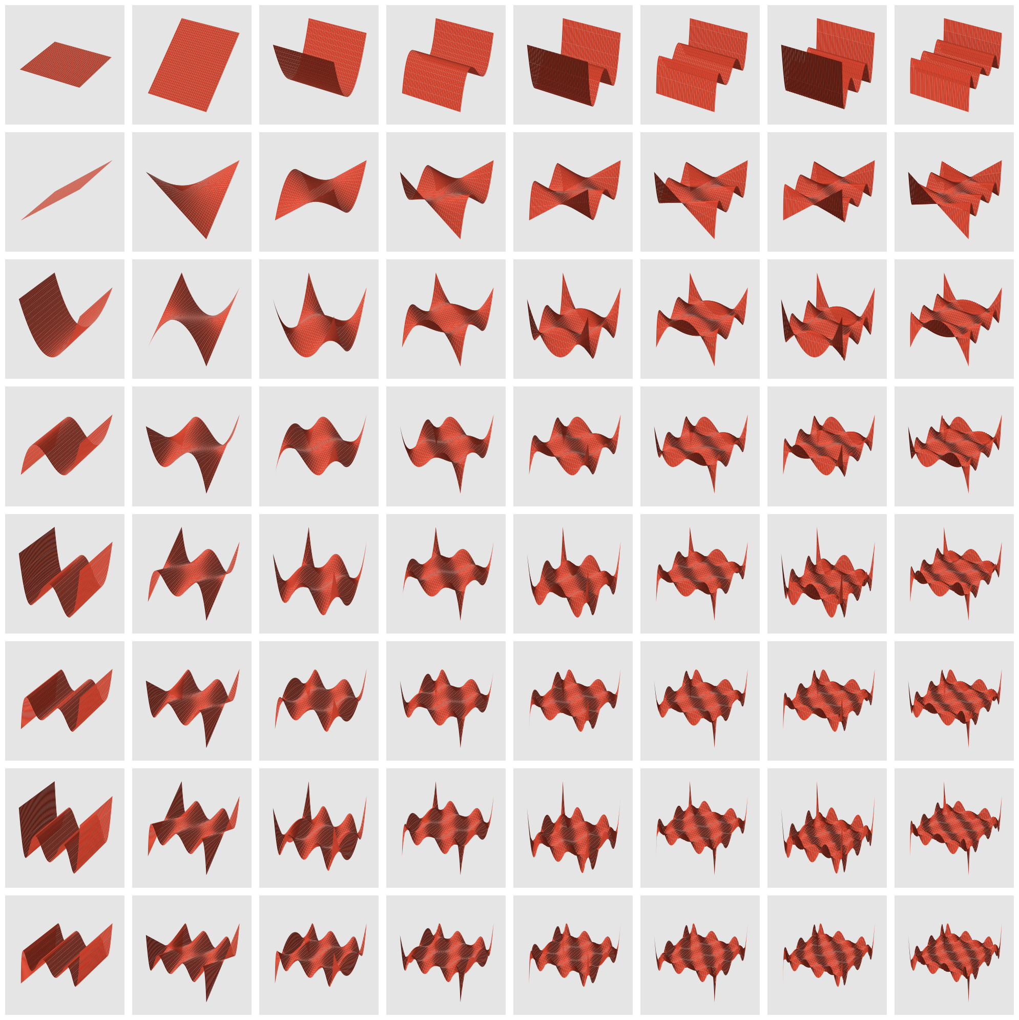
The image above suggests that large values of $m$ may be unstable, as the polynomials have large oscillations, while moderate values of $m$ will produce smooth basis functions.
We can now project any given $V_t$ into the space spanned by our basis functions. The best approximation $\hat{V}_t$ is
\[\hat V_t = \sum_{b=1}^B a_{t, b} \psi_b (x, y), \quad \quad \forall (x, y) \in \Omega,\]where the coefficients $a_{t, b}$ are estimated by minimizing the least square error,
\[a_t = \operatorname{argmin}_{\alpha} \sum_{i=1}^I \left( V_{t, i} - \sum_{b=1}^B \alpha_b \psi_b(x_i, y_i) \right)^2,\]where $\alpha_t \in \mathbb{R}^B$ is a vector with $B$ elements. We assume $I \gg B$ such that the problem above is well-posed. After this step, the original sequence of $V_t$ is replaced by a sequence of the projections $\hat V_t$.
To apply the Kahrunen-Loève decomposition, we express the basis functions $\varphi_\ell(x, y), \ell=1, \ldots, L$ as linear combination of the $\psi_b$ defined above,
\[\varphi_\ell(x, y) = \sum_{b=1}^B c_{\ell, b} \psi_b(x, y).\]Denoting $A = {A_{t, k}}$ the time series of the coefficients, with $A \in \mathbb{R}^{T, B}$, $\Psi(x, y) = (\psi_1(x, y), \ldots, \psi_B(x, y))$ the column vector of the $B$ basis functions and $c_\ell = (c_{\ell, 1}, \ldots, c_{\ell, B})$ the column vector of coefficients for the $\ell-th$ basis function, we obtain
\[\hat V(x, y) = A \Psi(x, y)\]and
\[\varphi_\ell(x, y) = \Psi(x, y)^T c_\ell.\]From the $T$ observation we can empirically estimate the covariance function with a simple averaging,
\[\hat C(x, y, u, v) = \frac{1}{T}\Psi(x, y)^T A^T A \Psi(u, v),\]where we have assumed for simplicity of exposition that the observations have zero mean.
Since each $\varphi_\ell$ is an eigenfunction, we must have
\[\begin{aligned} \int_{-1}^1 \int_{-1}^1 \left[ \frac{1}{T}\Psi(x, y)^T A^T A \Psi(u, v) ds dt \right] \Psi(u, v)^T c_\ell & = \lambda_\ell \Psi(x, y)^T c_\ell \\ % \frac{1}{T}\Psi(x, y)^T A^T A \int_{-1}^1 \int_{-1}^1 \Psi(u, v) \Psi(u, v)^T c_\ell ds dt & = \lambda_ \Psi(x, y)^T c_\ell. \end{aligned}\]The integral can be easily computed because of the orthonormality of the basis functions $\psi_\ell$, giving
\[\frac{1}{T}\Psi(x, y)^T A^T A c_\ell = \lambda_\ell \Psi(x, y)^T c_\ell, \quad \quad \forall x,y \in \Omega\]that is,
\[\frac{1}{T} A^T A c_\ell = \lambda_\ell c_\ell,\]which yields the $\ell-th$ eigenvalue and eigenvector of $A^T A$, where the eigenvalues are in decreasing ordered. Once the coefficients $c_\ell$ are computed, we can easily assemble $\varphi_\ell(x, y)$ as a linear composition of $\psi_b(x)$; the eigenvalues $\lambda_\ell$ will give their relative importance in explaning the variance, meaning that we can select the value $L$ that explains a predefined level of variance, say 99% or 99.5%.
Once computed the $\varphi_\ell$, the main result of the Kahrunen-Loève decomposition is that each $V_t$ can be written as a sum of its components, each ordered by the amount of variance it explains. This allows us to write
\[\hat V_t(x, y) = \sum_{\ell=1}^L v_{i, \ell} \varphi_\ell(x, y),\]where for a given value of $L$ the coefficients $v_{i, \ell}$ can be determined, in a similar way to what was done before, using a least-square approach.
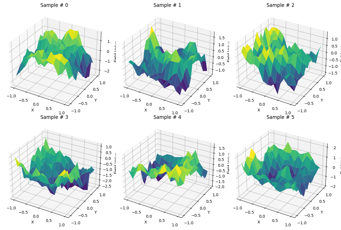
To apply the method just described we use a simple two-dimensional Gaussian process on the unitary square.
from scipy.linalg import cholesky

mean, sigma, w = 0.0, 1.0, 1.0

X, Y = np.meshgrid(np.linspace(-1, 1, 13), np.linspace(-1, 1, 17), indexing='ij')
points = np.column_stack([X.ravel(), Y.ravel()])

# covariance function
def covariance(p1, p2):
    x1, y1 = p1
    x2, y2 = p2
    dx = abs(x1 - x2)
    dy = abs(y1 - y2)
    return (sigma**2) * np.exp(-np.sqrt(dx**2 + dy**2) / w)

# compute the covariance matrix
N = points.shape[0]
cov_matrix = np.zeros((N, N))
for i in range(N):
    for j in range(N):
        cov_matrix[i, j] = covariance(points[i], points[j])

# cholesky decomposition of the covariance matrix
lower_chol = cholesky(cov_matrix, lower=True)

V_all = []
for _ in range(100):
    V_all.append(mean + np.dot(lower_chol, np.random.randn(N)).reshape(X.shape))
V_all = np.array(V_all)
We visualize a few entries to get a feeling of how they look like.
plt.style.use('default')
fig = plt.figure(figsize=(12, 8))
for i in range(6):
    ax = fig.add_subplot(2, 3, i + 1, projection='3d')
    ax.plot_surface(X, Y, V_all[i], cmap='viridis')
    ax.set_title(f'Sample # {i}')
    ax.set_xlabel('X')
    ax.set_ylabel('Y')
    ax.set_zlabel('Field Value')

plt.tight_layout()
Class LegendreProjection defines the $B$ basis functions on a given grid. Method transform() takes in input the $V_t$ and returns the coefficients of the each entry in terms of our Legendre polynomials, while inverse_transform() performs the opposite.
from sklearn.linear_model import LinearRegression


class LegendreProjection:

    def __init__(self, x_grid, y_grid, max_polynomial_order):
        self.ψ_all = []
        self.order = []

        for i in range(1, max_polynomial_order + 1):
            for j in range(i + 1):
                temp = lambda x, y, j=j, i=i: \
                    eval_legendre(j, x) / np.sqrt(2 / (2 * j + 1)) * \
                    eval_legendre(i - j, y) / np.sqrt(2 / (2 * (i - j) + 1))

                self.ψ_all.append(temp)
                self.order.append([j, i - j])

        self.B = len(self.ψ_all)
        self.Ψ = lambda x, y: np.array([self.ψ_all[i](x, y) for i in range(self.B)])
        self.x_grid = x_grid
        self.y_grid = y_grid

    def fit(self, X):
        pass

    def transform(self, X):
        values = self.Ψ(self.x_grid.flatten(), self.y_grid.flatten()).T

        X_hat = []
        for X_i in X:
            reg = LinearRegression().fit(values, X_i.reshape(-1))
            X_hat.append([reg.intercept_] + reg.coef_.tolist())
        return np.array(X_hat)

    def inverse_transform(self, X_hat):
        X = []
        for X_hat_i in X_hat:
            X.append(self.value(X_hat_i))
        return np.array(X)

    def fit_transform(self, X):
        self.fit(X)
        return self.transform(X)

    def value(self, coeffs):
        retval = np.ones_like(self.x_grid) * coeffs[0]
        for i in range(len(self.ψ_all)):
            retval += coeffs[i + 1] * self.ψ_all[i](self.x_grid, self.y_grid)
        return retval
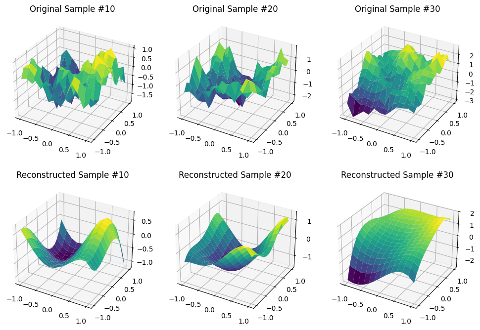
We will use $m=4$, which translates into $B=15$.
projection = LegendreProjection(X, Y, 4)
A = projection.fit_transform(V_all)
V_hat_all = projection.inverse_transform(A)
fig, axes = plt.subplots(figsize=(12, 8), nrows=2, ncols=3, subplot_kw=dict(projection='3d'))

axes[0, 0].set_title('Original Sample #10')
axes[0, 0].plot_surface(X, Y, V_all[10], cmap='viridis')
axes[1, 0].set_title('Reconstructed Sample #10')
axes[1, 0].plot_surface(X, Y, V_hat_all[10], cmap='viridis')

axes[0, 1].set_title('Original Sample #20')
axes[0, 1].plot_surface(X, Y, V_all[20], cmap='viridis')
axes[1, 1].set_title('Reconstructed Sample #20')
axes[1, 1].plot_surface(X, Y, V_hat_all[20], cmap='viridis')

axes[0, 2].set_title('Original Sample #30')
axes[0, 2].plot_surface(X, Y, V_all[30], cmap='viridis')
axes[1, 2].set_title('Reconstructed Sample #30')
axes[1, 2].plot_surface(X, Y, V_hat_all[30], cmap='viridis');
The FDA projection itself is a composition of the Legendre projection class and the remainder of the algorithm. The core part is the eigenproblem with the approximated covariance matrix (of the Legendre coefficients).
class FDAProjection:

    def __init__(self, x_grid, y_grid, max_polynomial_order):
        self.x_grid = x_grid
        self.y_grid = y_grid
        self.legendre = LegendreProjection(x_grid, y_grid, max_polynomial_order)

    def fit(self, samples):
        A = self.legendre.fit_transform(samples)
        A_mean = np.mean(A, axis=0)
        mean = lambda x, y, mean=A_mean: mean[0] + \
            np.sum([mean[j + 1] * self.legendre.ψ_all[j](x, y) for j in range(len(self.legendre.ψ_all))], axis=0)

        self.mean = mean
        A_zero_mean = A - A_mean

        A2 = 1.0 / A_zero_mean.shape[0] * A_zero_mean.T @ A_zero_mean
        self.K = A2.shape[0]
        if (cond := np.linalg.cond(A2)) > 1_000:
            print(f'Warning: matrix has condition number {cond}')
        self.λ_all, self.c_all = np.linalg.eig(A2)

        self.φ_all = []

        for i in range(len(self.λ_all)):
            self.φ_all.append(lambda x,y,i=i : self.c_all[0,i] + np.sum([self.c_all[j + 1, i] * self.legendre.ψ_all[j](x,y) for j in range(len(self.legendre.ψ_all))], axis=0))

        return A

    def transform(self, sample):
        X_flat = self.x_grid.flatten()
        Y_flat = self.y_grid.flatten()
        Z_flat = sample.flatten()

        basis_value = np.zeros((len(X_flat), self.K))
        for i in range(self.K):
            basis_value[:,i] = self.φ_all[i](X_flat, Y_flat)

        mean = self.mean(X_flat, Y_flat).reshape(-1, 1)
        Z_flat_zero_mean = Z_flat - mean.flatten()
        reg = LinearRegression(fit_intercept=False).fit(basis_value, Z_flat_zero_mean)
        return reg.coef_

    def inverse_transform(self, X_hat, L):
        X = self.mean(self.x_grid, self.y_grid)
        for i in range(L):
            X += X_hat[i] * self.φ_all[i](self.x_grid, self.y_grid)
        return X
fda = FDAProjection(X, Y, 4)
coeffs = fda.fit(V_all)
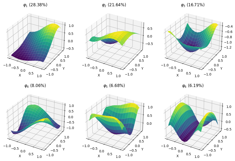
It is instructive to plot the basis functions of the covariance operator and the percentage of variance they explain.
plt.style.use('default')
fig = plt.figure(figsize=(12, 8))
for i in range(6):
    ax = fig.add_subplot(2, 3, i + 1, projection='3d')
    ax.plot_surface(X, Y, fda.φ_all[i](X, Y), cmap='viridis')
    ratio = fda.λ_all[i] / np.sum(fda.λ_all)
    ax.set_title(f'$φ_{i + 1}$ ({ratio:.2%})')
    ax.set_xlabel('X')
    ax.set_ylabel('Y')
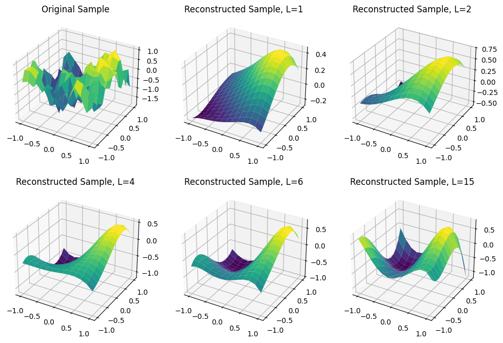
As expected, as $L$ increases the quality of the fit improves. With $L=15$ we have the same quality of the Legendre projection itself, since the $\varpi_\ell$ are linear combinations of the $\psi_b$ functions, but in this case there will be no dimensionality reduction.
fig, axes = plt.subplots(figsize=(12, 8), nrows=2, ncols=3, subplot_kw=dict(projection='3d'))

axes[0, 0].set_title('Original Sample')
axes[0, 0].plot_surface(X, Y, V_all[10], cmap='viridis')
axes[0, 1].set_title('Reconstructed Sample, L=1')
axes[0, 1].plot_surface(X, Y, fda.inverse_transform(fda.transform(V_hat_all[10]), 1), cmap='viridis')

axes[0, 2].set_title('Reconstructed Sample, L=2')
axes[0, 2].plot_surface(X, Y, fda.inverse_transform(fda.transform(V_hat_all[10]), 2), cmap='viridis')
axes[1, 0].set_title('Reconstructed Sample, L=4')
axes[1, 0].plot_surface(X, Y, fda.inverse_transform(fda.transform(V_hat_all[10]), 4), cmap='viridis')

axes[1, 1].set_title('Reconstructed Sample, L=6')
axes[1, 1].plot_surface(X, Y, fda.inverse_transform(fda.transform(V_hat_all[10]), 6), cmap='viridis')
axes[1, 2].set_title('Reconstructed Sample, L=15')
axes[1, 2].plot_surface(X, Y, fda.inverse_transform(fda.transform(V_hat_all[10]), 15), cmap='viridis');
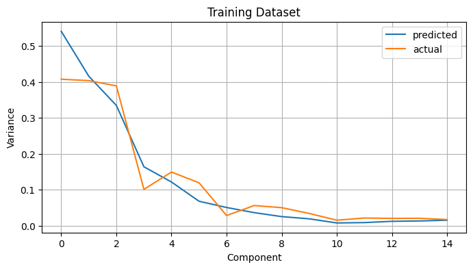
To finish, we compare the variance given by the eigenvalues $\lambda_\ell$ of the $\frac{1}{T} A^T A$ matrix and the actual variance of the projected components. They should be similar, and they appear to be.
plt.figure(figsize=(8, 4))
plt.plot(fda.λ_all, label='predicted')
plt.plot(np.var(coeffs, axis=0), label='actual')
plt.legend()
plt.xlabel('Component')
plt.ylabel('Variance')
plt.title('Training Dataset')
plt.grid();