The local volatility model is a popular model that allows pricing path-dependent options consistently with vanilla and other path-independent options. Developed through the works of Dupire and Derman and Kani, the local volatility model can be seen as an extension of the Black-Scholes model, where the time-dependent volatility $\sigma(t)$ is replaced by a function $\sigma_{loc}(x, t)$ that depends on both the asset level and the time.
Given the current spot value $S_0$, the SDE describing this model is
\[\begin{aligned} dX(t) & = \left( \mu - \frac{1}{2}\sigma_{loc}(X(t), t)^2 \right) + \sigma_{loc}(X(t), t) dW(t) \\ % X(0) & = X_0 = \log S_0. \end{aligned}\]The transitional probability distribution $p(x, t)$ describing the evolution of the probability distribution of a particle that is located at $X_0$ at $t=0$ is given by the famous Fokker-Planck equation,
\[\begin{aligned} \frac{\partial p(x, t)}{\partial t} & = -\frac{\partial}{\partial x}\left( \left( \mu - \frac{1}{2}\sigma_{loc}(X(t), t)^2 \right) p(x, t) \right) + \frac{\partial^2}{\partial x^2}\left( \frac{1}{2} \sigma_{loc}(X(t), t)^2 p(x, t) \right) \\ %% p(x, 0) & = \delta(x - X_0). \end{aligned}\]In this article we will solve the above equation, using the local volatility formulation provided by SSVI, using the same date of the SSVI article. We won’t calibrate SSVI here and simply take the calibrated parameters, that is η = 1.5830, λ = 0.3818, and ρ = -0.1332. To make things a bit simpler, the interest rates are assumed constant; at 5% and 3% they are roughly equivalent to real 2008 market data, but the code is a bit easier to follow.
import matplotlib.pylab as plt
import numpy as np
import pandas as pd
from scipy.interpolate import interp1d, PchipInterpolator
from scipy.linalg import solve_banded
from scipy.optimize import root_scalar
from scipy.stats import norm
S_0, r, q = 1.5184, 0.05, 0.03
X_0 = np.log(S_0)
T_all = [0, 0.019230769, 0.038461538, 0.083333333, 0.166666667, 0.25, 0.5, 0.75, 1, 2, 5]
σ_ATM_all = np.array([0, 0.1100, 0.1040, 0.0970, 0.0965, 0.0953, 0.0933, 0.0925, 0.0918, 0.0895, 0.0895])
V_ATM_all = σ_ATM_all**2 * T_all
ψ = PchipInterpolator(T_all, V_ATM_all)
η = 1.5830
λ = 0.3818
ρ = -0.1332
We need two functions to describe the local volatility surface: compute_w() returns the total implied variance at logmoneyness $Y$ and expiry $T$, while get_local_vol() returns the local volatility, this time at logmoneyness $X$ and expiry $T$. Both formulae are taken here from the original SSVI paper.
def compute_w(Y, T, η, λ, ρ):
    θ = ψ(T)
    φ = η * np.power(θ, -λ)
    return θ / 2 * (1 + ρ * φ * Y + np.sqrt((φ * Y + ρ)**2 + (1 - ρ**2)))
def get_local_vol(X, T, η, λ, ρ, ΔT, ΔY):
    log_F = X_0 + (r - q) * T
    Y = X - log_F
    T = max(T, 1.001 * ΔT)
    w = compute_w(Y, T, η, λ, ρ)
    w_plus_ΔT = compute_w(Y, T + ΔT, η, λ, ρ)
    w_minus_ΔT = compute_w(Y, T - ΔT, η, λ, ρ)
    num = (w_plus_ΔT - w_minus_ΔT) / 2 / ΔT
    w_plus_ΔY = compute_w(Y + ΔY, T, η, λ, ρ)
    w_minus_ΔY = compute_w(Y - ΔY, T, η, λ, ρ)
    w_prime = (w_plus_ΔY - w_minus_ΔY) / 2 / ΔY
    w_second = (w_plus_ΔY - 2 * w + w_minus_ΔY) / ΔY**2
    den = 1 - w_prime / w * (Y + 1 / 4 * w_prime * (1 + 1 / 4 * w - Y**2 / w)) \
        + 1 / 2 * w_second
    return np.sqrt(num / den)
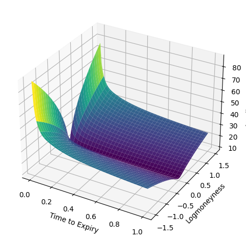
Y_all = np.linspace(-1.5, 1.5, 101)
T_all = np.linspace(1 / 256, 1, 101)
ZZ = []
for T in T_all:
    # Z_all = get_local_vol(Y_all, T, η, λ, ρ, 1e-5, 1e-5)
    Z_all = np.sqrt(compute_w(Y_all, T, η, λ, ρ) / T)
    ZZ.append(Z_all * 100)
XX, TT = np.meshgrid(Y_all, T_all)
ZZ = np.array(ZZ)
fig = plt.figure()
ax = plt.axes(projection='3d')
ax.plot_surface(TT, XX, ZZ, cmap='viridis')
ax.set_xlabel('Time to Expiry')
ax.set_ylabel('Logmoneyness')
ax.set_zlabel('Implied Vol (%)')
fig.tight_layout()
For the discretization of the Fokker-Planck equation requires we will use finite differences.
nx, nt = 1001, 1001
For the time axis, we use more nodes close to $t=0$, which is where the Dirac delta is located. The grid is built using a cosh transformation.
T_max = 1
T_axis = T_max * (np.cosh(np.linspace(0, 1, nt)) - 1)/ (np.cosh(1) - 1)
For the X-axis, instead, we follow the sinh formulae reported in the book Pricing Financial Instruments: The Finite Difference Method by Tavella and Randall, with the stretching coefficient here indicated as β and the concentration point set to be $\log(S_0)$. The X-axis covers six standard deviations when using the at-the-money volatility.
α = 6 * np.sqrt(compute_w(0.0, T_max, η, λ, ρ))
β = 0.1
X_min, X_max, X_star = X_0 - α, X_0 + α, X_0
c = np.arcsinh((X_max - X_star) / β)
d = np.arcsinh((X_min - X_star) / β)
ξ = np.linspace(0, 1, nx)
X_axis = X_star + β * np.sinh(c * ξ + d * (1 - ξ))
The time discretization is based on the θ-method, the space discretization on finite differences. Because the grid on the X-axis is non-uniform, we need to apply the first-order and second-order finite difference approximations for such grids. It is convenient to precompute the coefficients to speed up the calculations, which we do now.
ΔX = np.concatenate((np.diff(X_axis), [0]))
c_up, c_down, d_up, d_center, d_down = np.zeros(nx), np.zeros(nx), np.zeros(nx), np.zeros(nx), np.zeros(nx)
int_weights = np.zeros(nx)
for i in range(1, len(ΔX) - 1):
    c_up[i] = 1 / (ΔX[i] + ΔX[i - 1])
    c_down[i] = 1 / (ΔX[i] + ΔX[i - 1])
    scaling = 2 / (ΔX[i] + ΔX[i - 1])
    d_up[i] = scaling / ΔX[i]
    d_center[i] = scaling * (1 / ΔX[i] + 1 / ΔX[i - 1])
    d_down[i] = scaling  / ΔX[i - 1]
    int_weights[i] = (X_axis[i + 1] - X_axis[i - 1]) / 2
As it is well-known, the resulting linear system is tridiagonal. We use the solve_banded() function of scipy, which is quite parsimonious in terms of memory and computations. Only the diagonals are stored, see the official documentation for more details. Since we have zero Dirichlet boundary conditions, the first and last line of the matrix have a one on the diagonal and zero otherwise.
A = np.zeros((3, nx))
A[1, 0] = A[1, -1] = 1
A[0, 0] = A[0, 1] = 0
A[2, -2] = A[2, -1] = 0
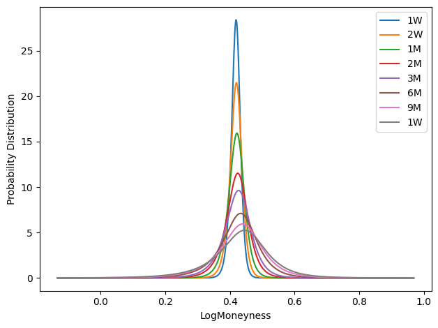
The loop below is quite classical; the only annoyance is the spikiness of the Dirac delta, which causes several problems to any solver. The Dirac delta itself is approximated by a Gaussian with variance ς, which is taken from our volatility surface at-the-money and with expiry of the first time step. It is also convenient to normalize the probabilities after each step.
ΔT = T_axis[1] - T_axis[0]
ς = compute_w(0, ΔT, η, λ, ρ)
p = 1 / np.sqrt(2 * np.pi * ς) * np.exp(-(X_axis - X_0)**2 / 2 / ς)
p /= sum(int_weights * p)

p_all = [p]
for n in range(len(T_axis) - 1):
    ΔT = T_axis[n + 1] - T_axis[n]
    diff_n = 0.5 * get_local_vol(X_axis, T_axis[n], η, λ, ρ, 1e-5, 1e-5)**2
    conv_n = r - q - diff_n

    diff_n1 = 0.5 * get_local_vol(X_axis, T_axis[n + 1], η, λ, ρ, 1e-5, 1e-5)**2
    conv_n1 = r - q - diff_n

    rhs = p.copy()
    θ = 1 if n < 2 else 1 / 2
    for i in range(1, nx - 1):
        A[0, i + 1] = θ * ΔT * (conv_n1[i + 1] * c_up[i] - diff_n1[i + 1] * d_up[i])
        A[1, i] = 1 + θ * ΔT * diff_n1[i] * d_center[i]
        A[2, i - 1] = θ * ΔT * (-conv_n1[i - 1] * c_down[i] - diff_n1[i - 1] * d_down[i])

        rhs[i] += -(1 - θ) * ΔT * (conv_n[i + 1] * c_up[i] - diff_n[i + 1] * d_up[i]) * p[i + 1]
        rhs[i] += -(1 - θ) * ΔT * diff_n[i] * d_center[i] * p[i]
        rhs[i] += -(1 - θ) * ΔT * (-conv_n[i - 1] * c_down[i] - diff_n[i - 1] * d_down[i]) * p[i - 1]

    p = solve_banded((1, 1), A, rhs)

    # normalize to have total probability of 1.0
    p /= sum(int_weights * p)
    p_all.append(p)
indices = [
    ('1W', np.searchsorted(T_axis, 1 / 52)),
    ('2W', np.searchsorted(T_axis, 2 / 52)),
    ('1M', np.searchsorted(T_axis, 1 / 12)),
    ('2M', np.searchsorted(T_axis, 2 / 12)),
    ('3M', np.searchsorted(T_axis, 3 / 12)),
    ('6M', np.searchsorted(T_axis, 6 / 12)),
    ('9M', np.searchsorted(T_axis, 9 / 12)),
    ('1W', np.searchsorted(T_axis, 1)),
]
fig = plt.figure()
for label, i in indices:
    plt.plot(X_axis, p_all[i], label=label)
plt.xlabel('LogMoneyness')
plt.ylabel('Probability Distribution')
plt.legend()
fig.tight_layout()
XX, TT = np.meshgrid(X_axis, T_axis)
ZZ = np.array(p_all)
plt.contourf(XX, TT, ZZ, levels=range(20))
plt.xlabel('LogMoneyness')
plt.ylabel('Time')
plt.title('Probability Distribution')
Text(0.5, 1.0, 'Probability Distribution')
We finish by comparing the implied volatilities computed by integrating the probability distributions we have just computed with those coming out of SSVI.
def compute_black_scholes_price(S_0, r, q, σ, K, T, is_call):
    assert T > 0
    ω = 1.0 if is_call else -1.0
    if T == 0.0:
        return max(ω * (S_0 - K), 0.0)
    df = np.exp(-r * T)
    F = S_0 * np.exp((r - q) * T)
    d_plus = (np.log(F / K) + 0.5 * σ**2 * T) / σ / np.sqrt(T)
    d_minus = d_plus - σ * np.sqrt(T)
    Φ = norm.cdf
    return ω * df * (F * Φ(ω * d_plus) - K * Φ(ω * d_minus))
def compute_implied_vol(S_0, r, q, σ_0, K, T, is_call , target_price):
    def inner(σ):
        return compute_black_scholes_price(S_0, r, q, σ, K, T, is_call) - target_price
    try:
        result = root_scalar(inner, x0=σ_0, bracket=[1e-3, 1])
    except:
        return np.nan
    return np.nan if not result.converged else result.root
def compute_smile(index):
    T = T_axis[index]
    σ_lv_all, σ_ssvi_all = [], []
    S_all = np.exp(X_axis)
    width = 3 * np.sqrt(compute_w(0.0, T, η, λ, ρ))
    S_min, S_max = S_0 * np.exp(-width), S_0 * np.exp(width)
    σ_lv_all, σ_ssvi_all = [], []
    for S in S_all:
        if S < S_min or S > S_max:
            σ_lv_all.append(np.nan)
            σ_ssvi_all.append(np.nan)
            continue
        K = S * np.exp((r - q) * T)
        is_call = K > S_0 * np.exp((r - q) * T)

        ω = 1.0 if is_call else -1.0
        price_lv = np.exp(-r * T) * sum(int_weights * p_all[index] * np.maximum(ω * (S_all - K), 0))
        σ_lv_all.append(compute_implied_vol(S_0, r, q, 0.1, K, T, is_call, price_lv))

        Y = np.log(K) - X_0 - (r - q) * T
        σ_ssvi_all.append(np.sqrt(compute_w(Y, T, η, λ, ρ) / T))
    return T, np.log(S_all), σ_lv_all, σ_ssvi_all
fig, axes = plt.subplots(figsize=(8, 16), nrows=4, ncols=2)
indices = [
    np.searchsorted(T_axis, 1 / 52),  # 1W
    np.searchsorted(T_axis, 2 / 52),  # 2W
    np.searchsorted(T_axis, 1 / 12),  # 1M
    np.searchsorted(T_axis, 2 / 12),  #
    np.searchsorted(T_axis, 3 / 12),
    np.searchsorted(T_axis, 6 / 12),
    np.searchsorted(T_axis, 9 / 12),
    np.searchsorted(T_axis, 1),
]
for index, ax in zip(indices, axes.flatten()):
    T, X_all, σ_lv_all, σ_ssvi_all = compute_smile(index=index)
    ax.plot(X_all, σ_lv_all, linewidth=8, alpha=0.25, label='LV')
    ax.plot(X_all, σ_ssvi_all, label='SSVI')
    ax.legend()
    ax.set_title(f'T = {T:.2f}')
fig.tight_layout()
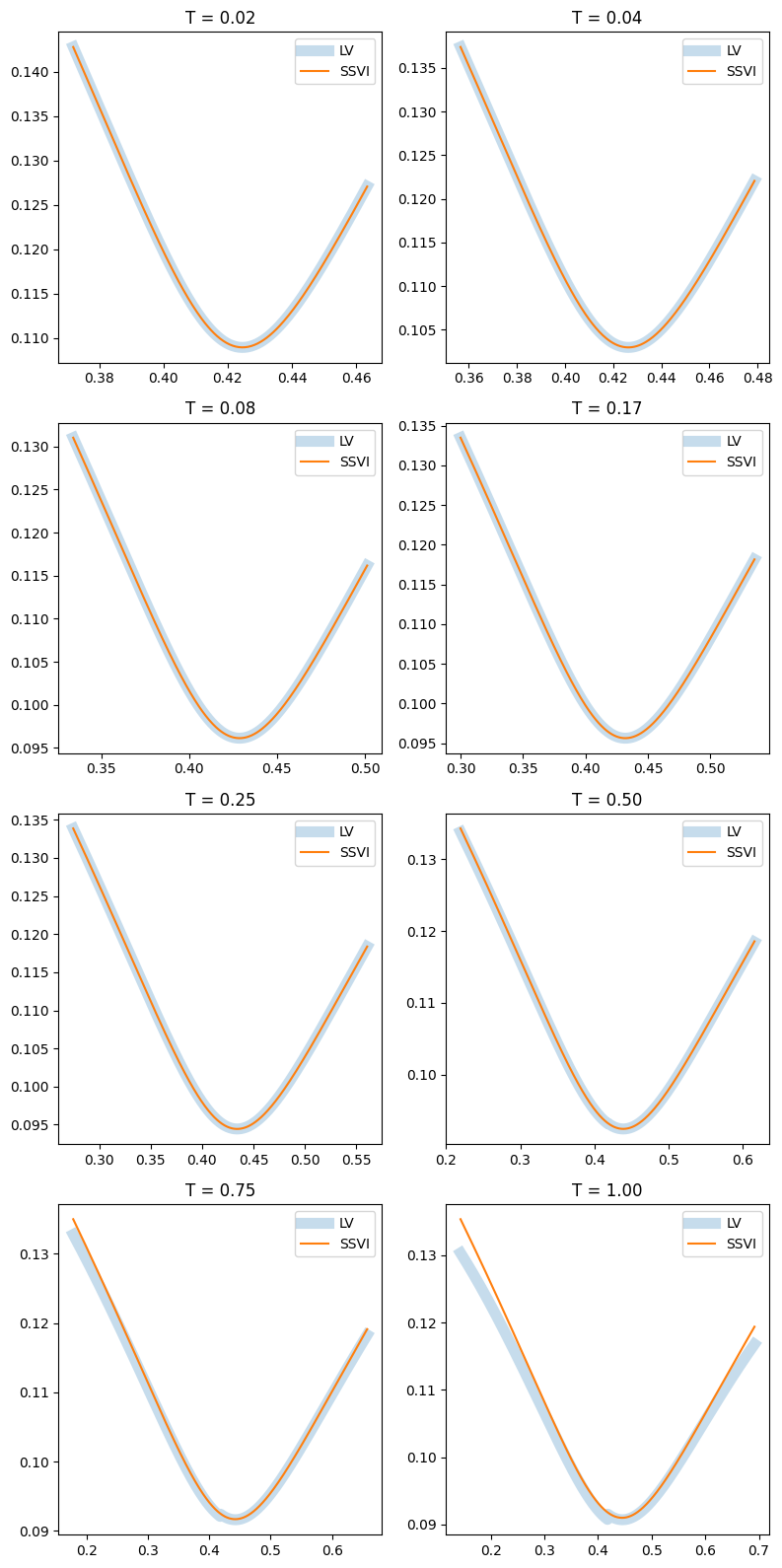
Results are quite good, with a small deterioration at one year. This is due to the grid concentration, which was needed for $t \approx 0$ but hot much for $t \gg 0$. Several solutions are possible – for example, one could define a new grid after a certain time, say T=0.5, and project the computed solution onto a new grid.