In this article we aim to reproduce the results presented in the paper Variational Autoencoders: A Hands-Off Approach to Volatility, by Maxime Bergeron, Nicholas Fung, John Hull, and Zissis Poulos, where the authors apply variational autoencoders to implied volatility surfaces. We will not use real market data, but rather the Heston model, which was discussed in a previous article; in another article we have covered in variational autoencoders in depth, to which we refer for more details.
The procedure is composed by three parts:
- in the first part, we look at how to generate implied volatility surfaces for the Heston model using the python binding of https://www.quantlib.org/;
- in the second part, we create the dataset by generating a large number of such surfaces, using some predefined ranges for the Heston parameters;
- in the third part, we train the variational autoencoder and check the quality of the results.
This notebook was run using the following environment:
conda create --name volatility-surface-generator python==3.9 --no-default-packages -y
conda activate volatility-surface-generator
pip install torch numpy sk-learn scipy matplotlib torch torchvision seaborn QuantLib ipykernel nbconvert tqdm ipywidgets
In the first part we define some helper functions and classes to connect to QuantLib. The parameters for the Heston model are contained in a namedtuple; the QuantLib surfaces is created by the function generate_ql_surface(), while compute_smile() computes a smile in strike space for a given maturity.
from collections import namedtuple
import numpy as np
from pathlib import Path
import QuantLib as ql
from matplotlib import cm
from matplotlib import pyplot as plt
import matplotlib.colors as mcolors
from mpl_toolkits.mplot3d import Axes3D
from scipy.stats import norm
Φ = norm.cdf
Model = namedtuple('Model', 'model_date, S_0, r, q, V_0, κ, θ, ζ, ρ')
def generate_ql_surface(model):
    # model coefficients
    model_date, S_0, r, q, V_0, κ, θ, ζ, ρ = model
    # rates and dividends, constant
    r_ts = ql.YieldTermStructureHandle(ql.FlatForward(model_date, r, ql.Actual365Fixed()))
    q_ts = ql.YieldTermStructureHandle(ql.FlatForward(model_date, q, ql.Actual365Fixed()))
    # Heston process, all params constant
    process = ql.HestonProcess(r_ts, q_ts, ql.QuoteHandle(ql.SimpleQuote(S_0)), V_0, κ, θ, ζ, ρ)
    heston_model = ql.HestonModel(process)
    heston_handle = ql.HestonModelHandle(heston_model)
    return ql.HestonBlackVolSurface(heston_handle)
The compute_smile function takes a built surface and looks at the at-the-money volatility for the specified expiry. Using this volatility it builds a vector of strikes that are close enough in probability to the forward, and computes the Black-Scholes implied volatility at those strikes. By default we do it with 101 points.
def compute_smile(model, ql_surface, period, factor=6, num_points=101):
    expiry_date = model.model_date + ql.Period(period)
    T = (expiry_date - model.model_date) / 365
    F = model.S_0 * np.exp((model.r - model.q) * T)
    σ_ATM = ql_surface.blackVol(expiry_date, F)
    width = factor * σ_ATM * np.sqrt(T)
    σ_all = []
    K_all = np.linspace(min(model.S_0, F) * np.exp(-width), max(model.S_0, F) * np.exp(width), num_points)
    for K in K_all:
        σ_all.append(ql_surface.blackVol(T, K))
    return T, F, K_all, σ_all
The small utility function get_date generates a random date in the QuantLib format. For what we do here the date is not important but it is still required by QuantLib.
def get_date():
    day = np.random.randint(1, 28)
    month = np.random.randint(1, 13)
    year = np.random.randint(2000, 2030)
    return ql.Date(day, month, year)
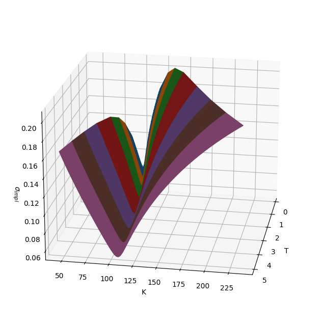
As an example, we visualize one such surface in strike and maturity space.
model = Model(get_date(), S_0=100.0, r=0.05, q=0.03, V_0=0.1**2, κ=0.25, θ=0.1**2, ζ=0.5, ρ=0.5)
ql_surface = generate_ql_surface(model)
X, Y, Z, C = [], [], [], []
colors = list(mcolors.TABLEAU_COLORS.values())
for color, period in zip(colors, ['1M', '3M', '6M', '1Y', '2Y', '3Y', '4Y', '5Y']):
    T, _, K_all, σ_all = compute_smile(model, ql_surface, period)
    X.append([T] * len(K_all))
    Y.append(K_all)
    Z.append(σ_all)
    C.append([color] * len(K_all))
fig, ax = plt.subplots(subplot_kw={'projection': '3d'}, figsize=(8, 8))
ax.plot_surface(np.array(X), np.array(Y), np.array(Z), facecolors=C)
ax.view_init(elev=20, azim=10, roll=0)
ax.set_xlabel('T')
ax.set_ylabel('K')
ax.set_zlabel('$σ_{impl}$');
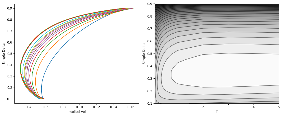
The problem with strikes is that they change for each maturity; they also depend on the volatility itself, while we would prefer a fixed grid as input to the autoencoder. To do that, we use deltas instead of strikes. The delta can be roughly interpreted as the probability of the option of ending up in-the-money. The delta can be defined in several ways; here we will use the so-called simple delta,
\[\delta = \Phi\left( \frac{\log\frac{F}{K}}{\sigma \sqrt{T} } \right),\]where $T$ is the option expiry, F$ is the forward at $T$, and $\sigma$ the implied volatility defined by the surface itself.
This is done by the compute_simple_delta_surface function below.
def compute_simple_delta_surface(model, num_deltas, periods):
    ql_surface = generate_ql_surface(model)
    d_grid = np.linspace(0.1, 0.9, num_deltas)
    X, Y, Z = [], [], []
    for period in periods:
        # compute on a strike grid
        T, F, K_all, σ_all = compute_smile(model, ql_surface, period)
        # interpolate on the simple delta grid
        d_all = Φ(np.log(K_all / F) / σ_all / np.sqrt(T))
        σ_grid = np.interp(d_grid, d_all, σ_all)
        # add to result
        X.append([T] * len(σ_grid))
        Y.append(d_grid)
        Z.append(σ_grid)
    return np.array(X), np.array(Y), np.array(Z)
model = Model(get_date(), S_0=1.0, r=-0.05, q=0.0, V_0=0.1**2, κ=0.25, θ=0.1**2, ζ=1, ρ=0.8)
periods = ['1M', '2M', '3M', '4M', '5M', '6M', '7M', '8M', '9M', '1Y', '2Y', '3Y', '4Y', '5Y']
X, Y, Z = compute_simple_delta_surface(model, 51, periods)
print(f'Surface shape: {Z.shape[0]}x{Z.shape[1]}')
fig, (ax0, ax1) = plt.subplots(figsize=(12, 5), ncols=2)
for y, z in zip(Y, Z):
    ax0.plot(z, y)
ax0.set_xlabel('Implied Vol'); ax0.set_ylabel('Simple Delta')
ax1.contour(X, Y, Z, colors='k', levels=25, alpha=0.5)
ax1.contourf(X, Y, Z, cmap='binary', levels=25)
ax1.set_xlabel('T'); ax1.set_ylabel('Simple Delta')
fig.tight_layout()
Surface shape: 14x51
We are ready for the second part. The Heston model depends on seven parameters, for which we define the following bounds:
- for the domestic interest rate, we take $r \in [-0.05, 0.05]$;
- for the continuously compounded dividends, we take $q \in [-0.05, 0.05]$;
- for the square root of the initial variance $V_0$, we have $\sqrt{V_0} \in [0.01, 0.5]$;
- for the mean reversion, we use $\kappa \in [0.05, 2]$;
- for the square root of the long-term variance, we consider $\sqrt{\theta} \in [0.01, 0.5]$;
- for the volatility of the variance process, we use $\zeta \in [0.01, 3]$;
- for the correlation, we take $\rho \in [-0.5, 0.5]$.
from scipy.stats import qmc, uniform
from tqdm import tqdm, trange
import pickle
bounds = np.array([
    [-0.01, 0.01],  # r
    [-0.01, 0.01],  # q
    [0.01, 0.5],  # sqrt(V_0)
    [0.05, 2.0],  # κ
    [0.01, 0.5],  # sqrt(θ)
    [0.01, 3],  # ζ
    [-0.5, +0.5],  # ρ
])
We use Sobol sequences to span through this sever-dimensional space. For each combination of the parameters, we need to sample the surface over some deltas and maturities. For the detlas, we use $\mathfrak{D} = { \delta_1, \ldots, \delta_d }$,with $\delta_1 = 0.1$, $\delta_d$ = 0.9, and the other points equally spaced, with $d=12$. This number is a bit small; much larger samples are needed for better results but we limit ourselves to small sample sizes.
For the maturities, we take $\mathfrak{M} = { \texttt{1M}, \texttt{2M}, \texttt{3M}, \texttt{4M}, \texttt{5M}, \texttt{6M}, \texttt{7M}, \texttt{8M}, \texttt{9M}, \texttt{1Y}, \texttt{18M}, \texttt{2Y}, \texttt{3Y}, \texttt{4Y}, \texttt{5Y} }$. The resulting surface is defined on a space $\mathfrak{Z} = \mathfrak{D} \times \mathfrak{M}$ and has dimension $20 \times 15 = 300$.
sobol = qmc.Sobol(d=7, scramble=False)
W_all = sobol.random_base2(m=12)
W_all = qmc.scale(W_all, bounds[:, 0], bounds[:, 1])
print(f'Generated {len(W_all)} entries.')
Generated 4096 entries.
periods = ['1M', '2M', '3M', '6M', '9M', '1Y', '2Y', '3Y']

model_date = get_date()
num_deltas = 5
num_tenors = len(periods)
filename = Path('surfaces.pickle')

import pickle
if filename.exists():
    with open(filename, 'rb') as f:
        params, XX, YY, surfaces = pickle.load(f)
        assert len(params) == len(surfaces)
        print(f'Read {len(surfaces)} surfaces.')
else:
    params, surfaces = [], []
    for r, q, sqrt_V_0, κ, sqrt_θ, ζ, ρ in tqdm(W_all):
        V_0 = sqrt_V_0**2
        θ = sqrt_θ**2
        # to limit by the Feller ratio
        # if κ * θ > ζ**2 / 2:
        model = Model(model_date, S_0=1, r=r, q=q, V_0=V_0, κ=κ, θ=θ, ζ=ζ, ρ=ρ)
        params.append((r, q, V_0, κ, θ, ζ, ρ))
        XX, YY, surface = compute_simple_delta_surface(model, num_deltas, periods)
        surfaces.append(surface)
    num_surfaces = len(surfaces)
    with open(filename, 'wb') as f:
        pickle.dump((params, XX, YY, surfaces), f)
surfaces = np.array(surfaces)
print(f'# surfaces: {num_surfaces}, min vol: {surfaces.min()}, max vol: {surfaces.max()}')
100%|██████████| 4096/4096 [01:46<00:00, 38.35it/s]

# surfaces: 4096, min vol: 0.0016473183503660689, max vol: 0.7606227339577064
We randomly split the generated data into a train dataset, containing 95% of the data, and a test dataset with the remainig 5% of the data. Using historical surfaces we would have split chronologically, however in this case a random split is enough.
from sklearn.model_selection import train_test_split
params_train, params_test, surfaces_train, surfaces_test = train_test_split(params, surfaces, test_size=0.05, random_state=42)
print(f"Using {len(surfaces_train)} for training and {len(surfaces_test)} for testing.")
Using 3891 for training and 205 for testing.
Although the numbers are already reasonably well scaled, being all in the range (0, 1), we make sure they are centered in zero and have unitary standard deviation.
class Scaler:

    def fit(self, X):
        self.mean = X.mean()
        self.std = X.std()

    def transform(self, X):
        return (X - self.mean) / self.std

    def inverse_transform(self, X):
        return X * self.std + self.mean

    def fit_transform(self, X):
        self.fit(X)
        return self.transform(X)
scaler = Scaler()
scaled_surfaces_train = scaler.fit_transform(surfaces_train)
scaled_surfaces_test = scaler.transform(surfaces_test)
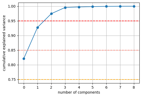
As baseline we use principal component analysis, or PCA. A few components are enough to take into account almost all variance, so we set of 9 components. The method as implemented by scikit-learn is extremely simple and fast. Even if the results of the PCA aren’t exceptionally good, its simplicity, speed and numerical robustness make it a very good baseline.
from sklearn.decomposition import PCA
PCA requires vectors, not matrices, therefore we need to flatten the data by lumping together the second and third dimensions.
X_train = np.array([k.flatten() for k in scaled_surfaces_train])
X_test = np.array([k.flatten() for k in scaled_surfaces_test])
num_components = 9
pca = PCA(n_components=num_components, whiten=False).fit(X_train)
plt.figure(figsize=(6, 4))
plt.plot(np.cumsum(pca.explained_variance_ratio_), 'o-')
plt.xlabel('number of components')
plt.ylabel('cumulative explained variance')
plt.axhline(y=0.75, linestyle='dashed', color='orange')
plt.axhline(y=0.85, linestyle='dashed', color='salmon')
plt.axhline(y=0.95, linestyle='dashed', color='red')
plt.grid();
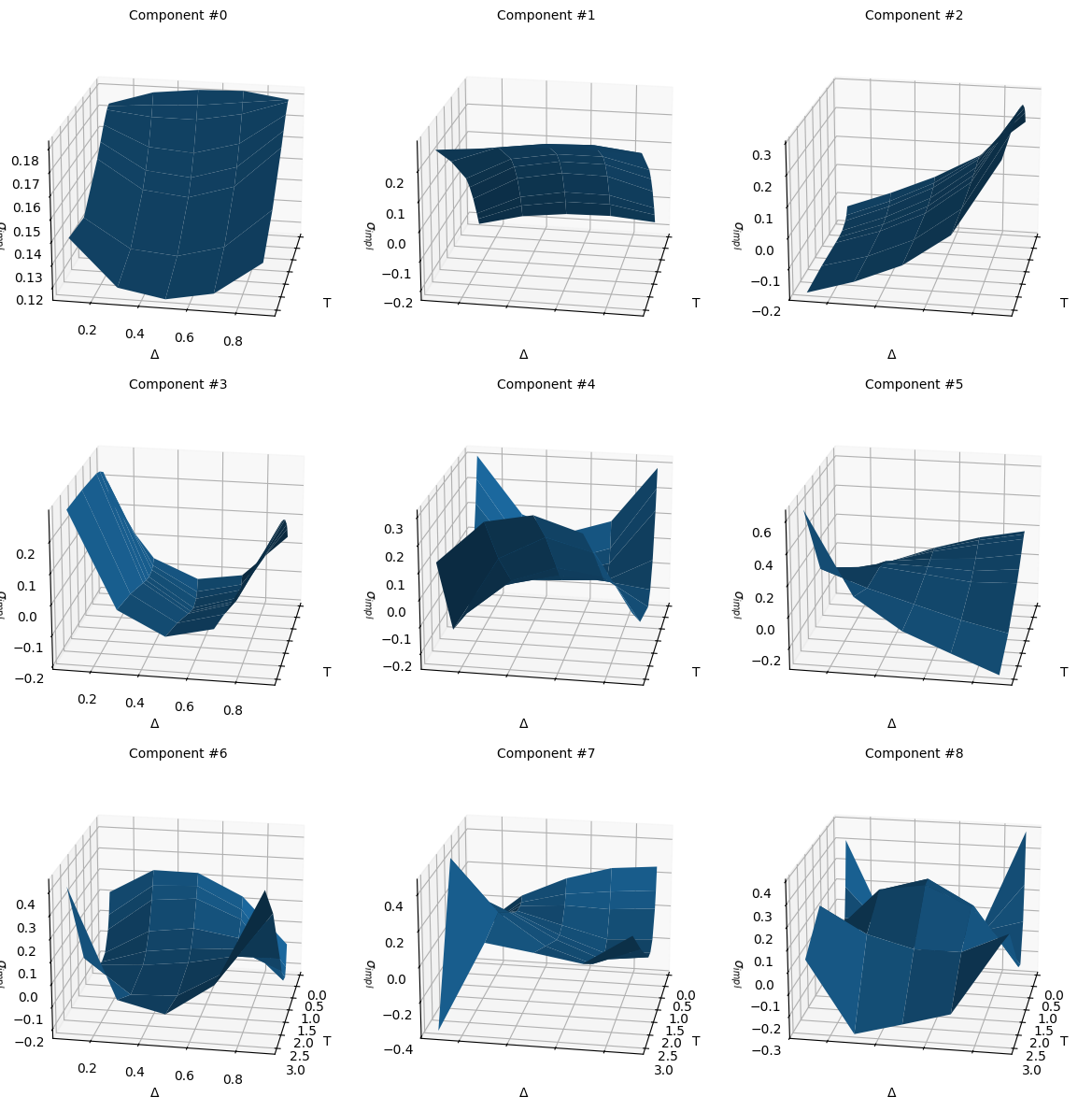
As seens in the visualizition below, components number 0 and 1 are the main shape of the surface, component number 2 is the skew in delta space, component number 3 the convexity in delta space, with the remaining ones giving the additional cross effects between the different parts of the surface.
components = pca.components_.reshape((-1, num_tenors, num_deltas))

fig, axes = plt.subplots(subplot_kw={'projection': '3d'},
                         figsize=(12, 12), nrows=3, ncols=3,
                         sharex=True, sharey=True)
axes = axes.flatten()
for i, ax in enumerate(axes.flatten()):
    ax.plot_surface(XX, YY, components[i])
    ax.view_init(elev=20, azim=10, roll=0)
    ax.set_xlabel('T')
    ax.set_ylabel('Δ')
    ax.set_zlabel('$σ_{impl}$');
    ax.set_title(f'Component #{i}', fontsize=10)
fig.tight_layout()
from sklearn.metrics import mean_absolute_error, mean_absolute_percentage_error
X_test_proj_pca = pca.inverse_transform(pca.transform(X_test))
surfaces_proj_pca = [scaler.inverse_transform(k.reshape(num_tenors, num_deltas)) for k in X_test_proj_pca]
mean_error_proj_pca = 10_000 * np.mean(abs(surfaces_test - surfaces_proj_pca), axis=0)
q95_error_proj_pca = 10_000 * np.quantile(abs(surfaces_test - surfaces_proj_pca), 0.95, axis=0)
max_error_proj_pca = 10_000 * np.max(abs(surfaces_test - surfaces_proj_pca), axis=0)

fig, (ax0, ax1, ax2) = plt.subplots(subplot_kw={'projection': '3d'}, figsize=(10, 6), ncols=3)

ax0.plot_surface(XX, YY, mean_error_proj_pca)
ax0.view_init(elev=20, azim=10, roll=0)
ax0.set_xlabel('T')
ax0.set_ylabel('Δ')
ax0.set_zlabel('Error (bps)');
ax0.set_title(f'Mean error: {mean_error_proj_pca.mean():.2f} (bps)')

ax1.plot_surface(XX, YY, q95_error_proj_pca)
ax1.view_init(elev=20, azim=10, roll=0)
ax1.set_xlabel('T')
ax1.set_ylabel('Δ')
ax1.set_zlabel('90% Quantile (%)');
ax1.set_title(f'Mean 95% quantile: {q95_error_proj_pca.max():.2f} (bps)')

ax2.plot_surface(XX, YY, max_error_proj_pca)
ax2.view_init(elev=20, azim=10, roll=0)
ax2.set_xlabel('T')
ax2.set_ylabel('Δ')
ax2.set_zlabel('Relative Error (%)');
ax2.set_title(f'Max error: {max_error_proj_pca.max():.2f} (bps)')

fig.tight_layout;

from scipy.optimize import minimize
def fit_pca(surface_target):
    surface_target = surface_target.flatten()

    def func(x):
        x_pred = scaler.inverse_transform(pca.inverse_transform(x))
        return np.linalg.norm(surface_target - x_pred)

    res = minimize(func, [0] * num_components, method='Powell')

    return scaler.inverse_transform(pca.inverse_transform(res.x)).reshape(num_tenors, num_deltas), res
errors_reconstr_pca = []
for surface_test in surfaces_test:
    surface_reconstr = fit_pca(surface_test)[0]
    errors_reconstr_pca.append(surface_reconstr - surface_test)
errors_reconstr_pca = np.array(errors_reconstr_pca).reshape(-1, num_tenors, num_deltas)
mean_error_reconstr_pca = 10_000 * np.mean(abs(errors_reconstr_pca), axis=0)
q95_error_reconstr_pca = 10_000 * np.quantile(abs(errors_reconstr_pca), 0.95, axis=0)
max_error_reconstr_pca = 10_000 * np.max(abs(errors_reconstr_pca), axis=0)
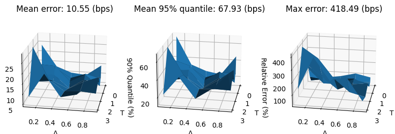
fig, (ax0, ax1, ax2) = plt.subplots(subplot_kw={'projection': '3d'}, figsize=(10, 6), ncols=3)
ax0.plot_surface(XX, YY, mean_error_reconstr_pca)
ax0.view_init(elev=20, azim=10, roll=0)
ax0.set_xlabel('T')
ax0.set_ylabel('Δ')
ax0.set_zlabel('Error (bps)');
ax0.set_title(f'Mean error: {mean_error_reconstr_pca.mean():.2f} (bps)')
ax1.plot_surface(XX, YY, q95_error_reconstr_pca)
ax1.view_init(elev=20, azim=10, roll=0)
ax1.set_xlabel('T')
ax1.set_ylabel('Δ')
ax1.set_zlabel('90% Quantile (%)');
ax1.set_title(f'Mean 95% quantile: {q95_error_reconstr_pca.max():.2f} (bps)')
ax2.plot_surface(XX, YY, max_error_reconstr_pca)
ax2.view_init(elev=20, azim=10, roll=0)
ax2.set_xlabel('T')
ax2.set_ylabel('Δ')
ax2.set_zlabel('Relative Error (%)');
ax2.set_title(f'Max error: {max_error_reconstr_pca.max():.2f} (bps)')
fig.tight_layout;
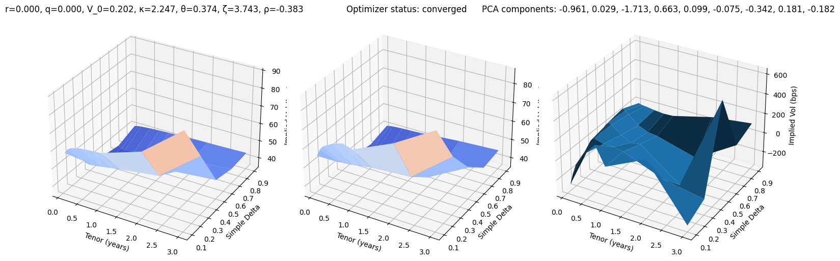
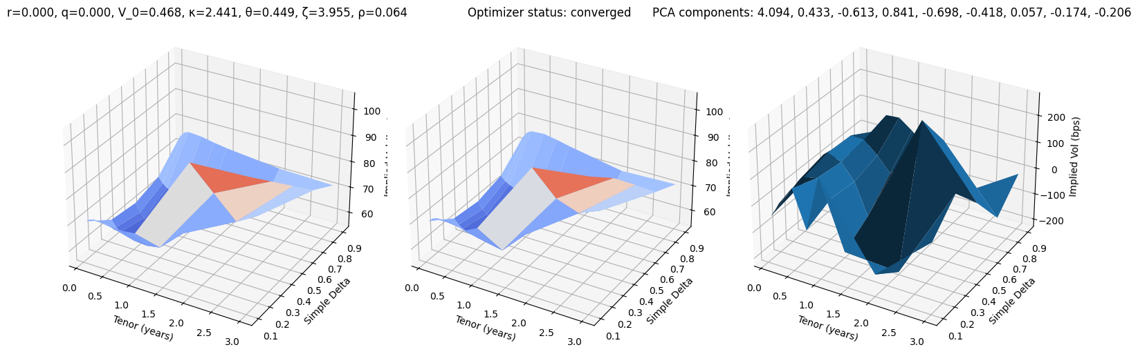
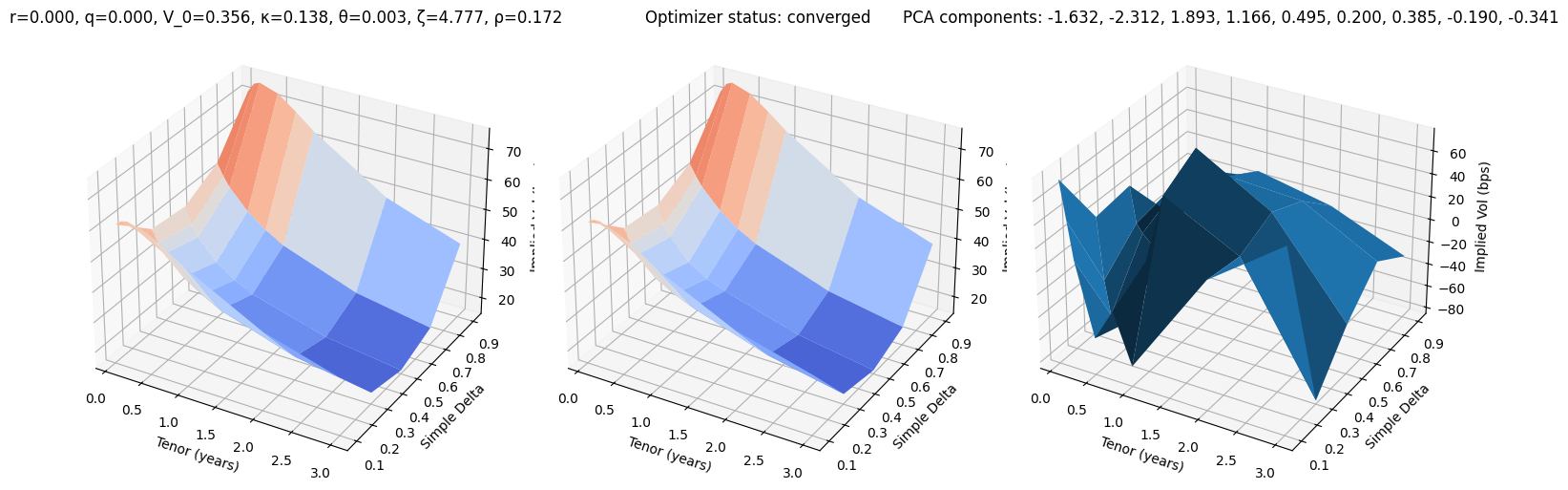
def test_pca(i):
    r, q, V_0, κ, θ, ζ, ρ = params_test[i]
    surface_target  = surfaces_test[i]

    surface_pca, res = fit_pca(surface_target)

    fig, (ax0, ax1, ax2) = plt.subplots(subplot_kw={'projection': '3d'}, figsize=(15, 5), ncols=3)
    vmin = 100 * min(surface_target.min(), surface_pca.min())
    vmax = 100 * max(surface_target.max(), surface_pca.max())
    ax0.plot_surface(XX, YY, 100 * surface_target, cmap=cm.coolwarm, norm=plt.Normalize(vmin, vmax))
    ax0.set_title(f"r={r:.3f}, q={q:.3f}, V_0={V_0:.3f}, κ={κ:.3f}, θ={θ:.3f}, ζ={ζ:.3f}, ρ={ρ:.3f}")
    ax1.plot_surface(XX, YY, 100 * surface_pca, cmap=cm.coolwarm, norm=plt.Normalize(vmin, vmax))
    ax1.set_title(f'Optimizer status: ' + 'converged' if res.success else 'not converged')
    ax2.set_title('PCA components: ' + ', '.join([f'{k:.3f}' for k in res.x]))
    error = 10_000 * surface_pca - 10_000 * surface_target
    ax2.plot_surface(XX, YY, error)
    for ax in (ax0, ax1, ax2):
        ax.set_xlabel('Tenor (years)'); ax.set_ylabel('Simple Delta'); ax.set_zlabel('Implied Vol (bps)')
    fig.tight_layout()
test_pca(10)
test_pca(20)
test_pca(30)
After having established a baseline, we are ready to start with the variational autoencoder.
import seaborn as sns
import torch
import torch.nn as nn
import torch.nn.functional as F
import torch.utils
import torch.distributions
from torch.utils.data import Dataset, DataLoader

torch.manual_seed(0)
torch.set_default_dtype(torch.float64)
device = 'cpu'
We reuse the code from the article on variational autoencoders, with tiny differences. One of them is the usage of $\beta$-VAE and different scaling for the loglikelihood.
class VariationalEncoder(nn.Module):

    def __init__(self, num_tenors, num_deltas, num_latent, num_hidden):
        super().__init__()
        self.num_points = num_tenors * num_deltas
        self.linear1 = nn.Linear(self.num_points, 4 * num_hidden)
        self.linear2 = nn.Linear(4 * num_hidden, 2 * num_hidden)
        self.linear3 = nn.Linear(2 * num_hidden, num_hidden)
        self.linear_mu = nn.Linear(num_hidden, num_latent)
        self.linear_logsigma2 = nn.Linear(num_hidden, num_latent)

    def forward(self, x):
        x = x.view(-1, self.num_points)
        x = F.tanh(self.linear1(x))
        x = F.tanh(self.linear2(x))
        x = F.tanh(self.linear3(x))
        mu =  self.linear_mu(x)
        logsigma2 = self.linear_logsigma2(x)
        sigma = torch.exp(0.5 * logsigma2)
        ξ = torch.randn_like(mu)
        z = mu + sigma * ξ
        kl = torch.mean(torch.sum((sigma**2 + mu**2 - logsigma2 - 1) / 2, dim=1), dim=0)
        return z, kl
class Decoder(nn.Module):

    def __init__(self, num_tenors, num_deltas, num_latent, num_hidden):
        super().__init__()
        self.num_deltas = num_deltas
        self.num_tenors = num_tenors
        self.linear1 = nn.Linear(num_latent, num_hidden)
        self.linear2 = nn.Linear(num_hidden, 2 * num_hidden)
        self.linear3 = nn.Linear(2 * num_hidden, 4 * num_hidden)
        self.linear4 = nn.Linear(4 * num_hidden, self.num_tenors * self.num_deltas)

    def forward(self, z):
        z = F.tanh(self.linear1(z))
        z = F.tanh(self.linear2(z))
        z = F.tanh(self.linear3(z))
        z = self.linear4(z)
        return z.view(-1, self.num_tenors, self.num_deltas)
class VariationalAutoencoder(nn.Module):

    def __init__(self, num_tenors, num_deltas, num_latent, num_hidden):
        super().__init__()
        self.num_latent = num_latent
        self.num_points = num_tenors * num_deltas
        self.encoder = VariationalEncoder(num_tenors, num_deltas, num_latent, num_hidden)
        self.decoder = Decoder(num_tenors, num_deltas, num_latent, num_hidden)

    def forward(self, x):
        z, kl = self.encoder(x)
        x_hat = self.decoder(z)
        return x_hat, kl

    def compute_log_likelihood(self, X, X_hat, η):
        X = X.view(-1, self.num_points)
        X_hat = X_hat.view(-1, self.num_points)
        ξ = torch.randn_like(X_hat)
        X_sampled = X_hat + η.sqrt() * ξ
        return 0.5 * F.mse_loss(X, X_sampled) / η + η.log()
As customary, we derive from the Torch’s Dataset class to wrap our training dataset.
class HestonDataset(Dataset):

    def __init__(self, X):
        self.X = X

    def __len__(self):
        return len(self.X)

    def __getitem__(self, idx):
        return torch.tensor(self.X[idx])
def train(vae, data, epochs=20, lr=1e-3, gamma=0.95, η=0.1, β_kl=1.0, print_every=1):
η = torch.tensor(η)
optimizer = torch.optim.RMSprop(vae.parameters(), lr=lr)
scheduler = torch.optim.lr_scheduler.ExponentialLR(optimizer, gamma=gamma)
history = []
for epoch in trange(epochs):
last_lr = scheduler.get_last_lr()
total_log_loss, total_kl_loss, total_loss = 0.0, 0.0, 0.0
for x in data:
x = x.to(device)
optimizer.zero_grad()
x_hat, kl_loss = vae(x)
log_loss = vae.compute_log_likelihood(x, x_hat, η)
loss = log_loss + β_kl * kl_loss
total_log_loss += log_loss.item()
total_kl_loss += β_kl * kl_loss.item()
total_loss += loss.item()
loss.backward()
optimizer.step()
scheduler.step()
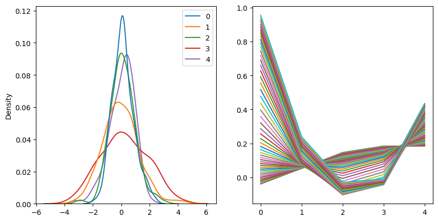
if (epoch + 1) % print_every == 0:
with torch.no_grad():
_, (ax0, ax1) = plt.subplots(figsize=(10, 5), ncols=2)
Z = vae.encoder(torch.tensor(scaled_surfaces_test).to(device))[0].cpu().detach().numpy()
sns.kdeplot(data=Z, ax=ax0)
for z in np.linspace(-3, 3):
z = [z] + [0.0] * (vae.num_latent - 1)
surface_vae = vae.decoder(torch.tensor(z).unsqueeze(0).to(device))[0].cpu().detach().numpy().reshape(num_tenors, num_deltas)
ax1.plot(surface_vae[0])
plt.show()
print(f"Epoch: {epoch + 1:3d}, lr=: {last_lr[0]:.4e}, " \
f"total log loss: {total_log_loss:.4f}, total KL loss: {total_kl_loss:.4f}, total loss: {total_loss:.4f}")
history.append((total_log_loss, total_kl_loss))
return np.array(history)
dataset = HestonDataset(scaled_surfaces_train)
data_loader = DataLoader(dataset, batch_size=128, shuffle=True)
def init_weights(m):
    if isinstance(m, nn.Linear):
        torch.nn.init.xavier_uniform_(m.weight)
        m.bias.data.fill_(0.01)
num_latent = 5
vae = VariationalAutoencoder(num_tenors, num_deltas, num_latent, num_hidden=32).to(device)
torch.manual_seed(0)
vae.apply(init_weights);
history = train(vae, data_loader, epochs=5_000, lr=5e-4, gamma=1, η=0.01, β_kl=1e-3, print_every=5_000)
100%|█████████▉| 4998/5000 [02:51<00:00, 30.53it/s]
100%|██████████| 5000/5000 [02:51<00:00, 29.11it/s]

Epoch: 5000, lr=: 5.0000e-04, total log loss: -125.6315, total KL loss: 0.6787, total loss: -124.9528
def fit_vae(surface_target):
    def func(x):
        surface_pred = scaler.inverse_transform(vae.decoder(torch.tensor(x).unsqueeze(0).to(device))[0])
        surface_pred = surface_pred.cpu().detach().numpy()
        diff = np.linalg.norm(surface_target.flatten() - surface_pred.flatten(), ord=np.inf)
        return diff

    best_res = None
    for method in ['Nelder-Mead', 'Powell', 'BFGS']:
        res = minimize(func, [0] * num_latent, method=method)
        if best_res is None or (res.fun < best_res.fun and res.success):
            best_res = res

    pred = vae.decoder(torch.tensor(best_res.x).unsqueeze(0).to(device))[0].cpu().detach().numpy().reshape(num_tenors, num_deltas)
    return scaler.inverse_transform(pred), best_res
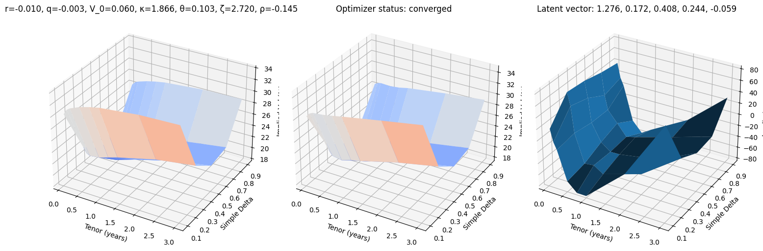
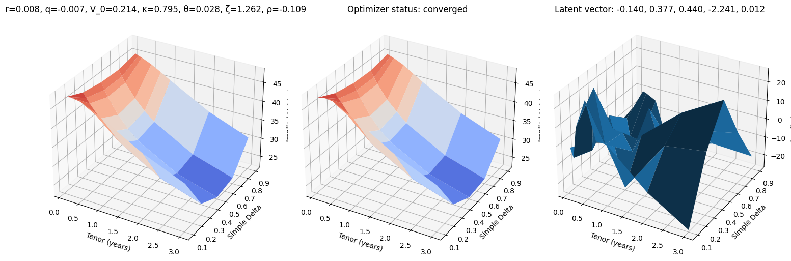
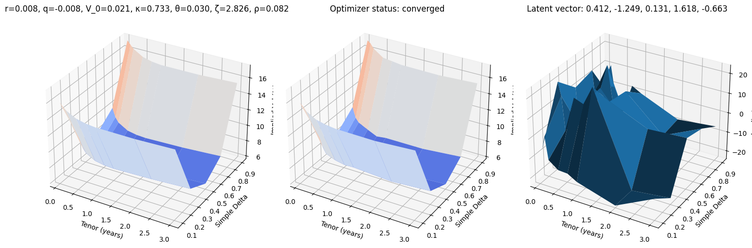
def test_vae(i, use_train=False):
    r, q, V_0, κ, θ, ζ, ρ = params_train[i] if use_train else params_test[i]
    surface_target  = surfaces_train[i] if use_train else surfaces_test[i]

    surface_vae, res = fit_vae(surface_target)

    fig, (ax0, ax1, ax2) = plt.subplots(subplot_kw={'projection': '3d'}, figsize=(15, 5), ncols=3)
    vmin = 100 * min(surface_target.min(), surface_vae.min())
    vmax = 100 * max(surface_target.max(), surface_vae.max())
    ax0.plot_surface(XX, YY, 100 * surface_target, cmap=cm.coolwarm, norm=plt.Normalize(vmin, vmax))
    ax0.set_title(f"r={r:.3f}, q={q:.3f}, V_0={V_0:.3f}, κ={κ:.3f}, θ={θ:.3f}, ζ={ζ:.3f}, ρ={ρ:.3f}")
    ax1.plot_surface(XX, YY, 100 * surface_vae, cmap=cm.coolwarm, norm=plt.Normalize(vmin, vmax))
    ax1.set_title(f'Optimizer status: ' + 'converged' if res.success else 'not converged')
    ax2.set_title('Latent vector: ' + ', '.join([f'{k:.3f}' for k in res.x]))
    error = 10_000 * surface_vae - 10_000 * surface_target
    ax2.plot_surface(XX, YY, error)
    for ax in (ax0, ax1, ax2):
        ax.set_xlabel('Tenor (years)'); ax.set_ylabel('Simple Delta'); ax.set_zlabel('Implied Vol (%)')
    fig.tight_layout()
test_vae(10)
test_vae(100)
test_vae(200)
errors_reconstr_vae = []
for surface_test in (pbar := tqdm(surfaces_test)):
    surface_reconstr = fit_vae(surface_test)[0]
    error = surface_reconstr - surface_test
    pbar.set_description(f'{abs(error).max():.2f}')
    errors_reconstr_vae.append(error)
errors_reconstr_vae = np.array(errors_reconstr_vae).reshape(-1, num_tenors, num_deltas)
0.00: 100%|██████████| 205/205 [00:23<00:00, 8.79it/s]
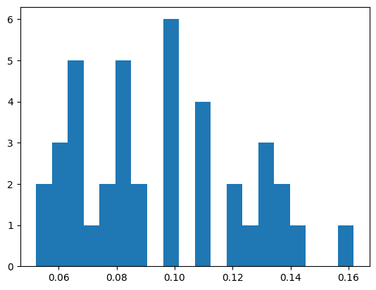
plt.hist(np.max(errors_reconstr_vae.reshape(205, -1), axis=0), bins=20);
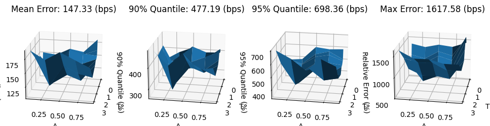
mean_error_reconstr_vae = 10_000 * np.mean(abs(errors_reconstr_vae), axis=0)
q90_error_reconstr_vae = 10_000 * np.quantile(abs(errors_reconstr_vae), 0.90, axis=0)
q95_error_reconstr_vae = 10_000 * np.quantile(abs(errors_reconstr_vae), 0.95, axis=0)
max_error_reconstr_vae = 10_000 * np.max(abs(errors_reconstr_vae), axis=0)

fig, (ax0, ax1, ax2, ax3) = plt.subplots(subplot_kw={'projection': '3d'}, figsize=(12, 6), ncols=4)

ax0.plot_surface(XX, YY, mean_error_reconstr_vae)
ax0.set_zlabel('Error (bps)');
ax0.set_title(f'Mean Error: {mean_error_reconstr_vae.mean():.2f} (bps)')

ax1.plot_surface(XX, YY, q90_error_reconstr_vae)
ax1.set_zlabel('90% Quantile (%)');
ax1.set_title(f'90% Quantile: {q90_error_reconstr_vae.max():.2f} (bps)')

ax2.plot_surface(XX, YY, q95_error_reconstr_vae)
ax2.set_zlabel('95% Quantile (%)');
ax2.set_title(f'95% Quantile: {q95_error_reconstr_vae.max():.2f} (bps)')

ax3.plot_surface(XX, YY, max_error_reconstr_vae)
ax3.set_zlabel('Relative Error (%)');
ax3.set_title(f'Max Error: {max_error_reconstr_vae.max():.2f} (bps)')

for ax in [ax0, ax1, ax2, ax3]:
    ax.view_init(elev=20, azim=10, roll=0)
    ax.set_xlabel('T')
    ax.set_ylabel('Δ')

fig.tight_layout;
Finally, we check the shape of the latent space on the training set. The pair plot shows the distribution of each latent variable on the diagonals and the scatter plots of two latent variables on the off-diagonal plots. On the upper triangular part we have superimposed the circles with the ideal distribution, while on the lower triangular part the lines show the actual isolines from the kernel density estimations.
import pandas as pd
from matplotlib.patches import Circle
Z = vae.encoder(torch.tensor(scaled_surfaces_test).to(device))[0].cpu().detach().numpy()
g = sns.pairplot(pd.DataFrame(Z, columns=[f"Z_{i}" for i in range(num_latent)]), diag_kind='kde', corner=False)
g.map_lower(sns.kdeplot, levels=4, color="orange")
for r in [1, 2, 3, 4]:
    for j in range(1, num_latent):
        for i in range(0, j):
            g.axes[i, j].add_patch(Circle((0, 0), r, linestyle='dashed', color='crimson', alpha=1, fill=None))
            g.axes[i, j].set_xlim(-4, 4)
            g.axes[i, j].set_ylim(-4, 4)
g.figure.tight_layout()
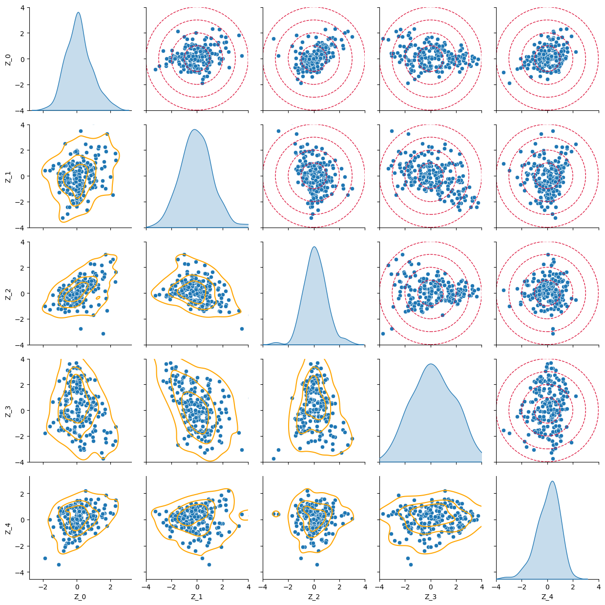
This shows that we can effectively generate Heston-type surfaces using variational autoencoders. The training dataset is of modest dimension – the quality of the reconstructed entities could be improved with more samples.